Directional quantile envelopes

Introduction

In this blog post I am going to discuss the computation of the so called directional quantile envelopes; see [5] for definitions, theorems, and concrete examples. The Mathematica package QuantileRegression.m, [1] has an experimental implementation, the function QuantileEnvelope.

This type of implementation investigation is a natural extension of the quantile regression implementations and utilization I have done before. (See the package [1] and the related guide [2]; blog posts [3,4].) I was looking for a 2D quantile regression technique that can be used as a tool for finding 2D outliers. From the exposition below it should be obvious that the technique can be generalized in higher dimensions.

The idea of directional quantile envelopes is conceptually simple (and straightforward to come up with). The calculation is also relatively simple: over a set of uniformly distributed directions we find the lines that separate the data according a quantile parameter q, 0<q<1, and with those lines we approximate the enveloping curve for data that corresponds to q.

The algorithm

Here is the full algorithm. (The figure below can be used as a visual aid).

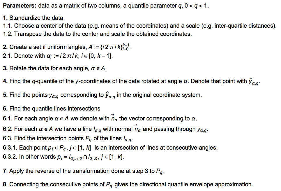
Parameters: data as a matrix of two columns, a quantile parameter q, 0<q<1.
1. Standardize the data.
1.1. Choose a center of the data (e.g. means of the coordinates) and a scale (e.g. inter-quartile distances).
1.2. Transpose the data to the center and scale the obtained coordinates.
2. Create a set of k uniform angles, A:={i2Pi/k}, 0<=i<=k-1 .
2.1. Denote with a[i]:=i2Pi/k, i∈[0,k-1].
3. Rotate the data for each angle, a[i]∈A.
4. Find the q-quantile of the y-coordinates of the data rotated at angle a. Denote that point with r[a,q].
5. Find the points y[a,q] corresponding to r[a,q] in the original coordinate system.
6. Find the quantile lines intersections
6.1. For each angle a∈A we denote with n[a] the vector corresponding to a.
6.2. For each a∈A we have a line l[a,q] with normal n[a] and passing through y[a,q].
6.3. Find the intersection points P[q] of the lines l[a,q].
6.3.1. Each point p[j]∈P[q], j∈[1,k] is an intersection of lines at consecutive angles.
6.3.2. In other words p[j]=l[a[j-1],q] ∩ l[a[j],q], j∈[1,k].
7. Apply the reverse of the transformation done at step 3 to P[q].
8. Connecting the consecutive points of P[q] gives the directional quantile envelope approximation.

Click this thumbnail for an image with better math notation:

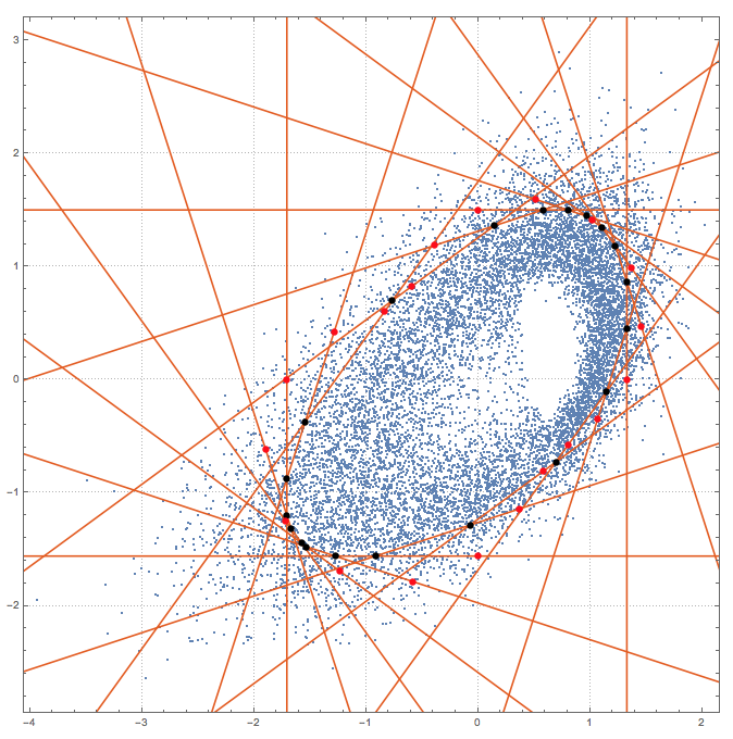
Algorithm visual aid

Here is an example of an application of the described algorithm. The points in blue are the data points, the points in red are the points y[a,q], the red lines are the lines l[a,q], the points in black are the points P.

Remarks

Remark 1: The function QuantileEnvelope of [1] follows the described algorithm. The rotations are done using matrix multiplication; the function Reduce is used to find the intersections between the lines.

Remark 2: A possible alternative algorithm is to use “the usual” quantile regression with polar coordinates. (The article [5] refers to and briefly discusses such an approach.)

Example data

In order to demonstrate the function QuantileEnvelope let us define a couple of data sets.

The first data set is generated with the function SkewNormalDistribution, so the data set name is sndData.

npoints = 12000;
data = {RandomReal[{0, 2 [Pi]}, npoints],
RandomVariate[SkewNormalDistribution[0.6, 0.3, 4], npoints]};
data = MapThread[#2*{Cos[#1], Sin[#1]} &, data];
rmat = RotationMatrix[-[Pi]/2.5].DiagonalMatrix[{2, 1}];
data = Transpose[rmat.Transpose[data]];
data = TranslationTransform[{-Norm[Abs[#]/3], 0}][#] & /@ data;
sndData = Standardize[data];

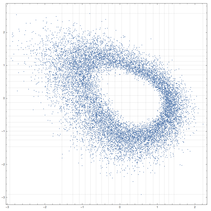
Here is a plot of sndData with grid lines derived from the quantiles of x and y coordinates of the data set.

ListPlot[sndData, PlotRange -> All, AspectRatio -> 1, PlotTheme -> "Detailed",
GridLines -> Map[Quantile[#, Range[0, 1, 1/19]] &, Transpose[sndData]],
ImageSize -> 700]

The second uses the function PoissonDistribution, so the data set name is pdData.

npoints = 12000;
data = RandomReal[NormalDistribution[12, 5.6], npoints];
data = Transpose[{data,
data + RandomVariate[PoissonDistribution[12], npoints] +
RandomReal[{-0.2, 0.2}, npoints]}];
data = Select[data, #[[2]] > 0 &];
data[[All, 2]] = Log[data[[All, 2]]];
pdData = data;

Here is a plot of pdData with grid lines derived from the quantiles of x and y coordinates of the data set.

ListPlot[pdData, PlotRange -> All, AspectRatio -> 1, PlotTheme -> "Detailed",
GridLines -> Map[Quantile[#, Range[0, 1, 1/19]] &, Transpose[pdData]],
ImageSize -> 700]

Examples of application (with QuantileEnvelope)

Let us demonstrate the function QuantileEnvelope. The function arguments are a data matrix, a quantile specification, and number of directions. The quantile specification can a number or a list of numbers. The function returns the intersection points of the quantile lines at different directions.

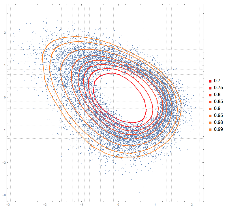
Here is an application to the dataset sndData over 8 different quantiles over 60 different uniformly spread directions.

In[630]:= qs = {0.7, 0.75, 0.8, 0.85, 0.90, 0.95, 0.98, .99} ;
AbsoluteTiming[qsPoints = QuantileEnvelope[sndData, qs, 60];]
Out[631]= {0.150104, Null}

The result is a list of 8 lists of 60 points.

In[632]:= Dimensions[qsPoints]
Out[632]= {8, 60, 2}

Let us plot the data and the direction quantile envelopes.

Block[{data = sndData},
Show[{ListPlot[data, AspectRatio -> 1, PlotTheme -> {"Detailed"},
GridLines ->
Map[Quantile[#, Range[0, 1, 1/(20 - 1)]] &, Transpose[data]],
PlotLegends ->
SwatchLegend[
Blend[{Red, Orange},
Rescale[#1, {Min[qs], Max[qs]}, {0, 1}]] & /@ qs, qs]],
Graphics[{PointSize[0.005], Thickness[0.0025],
MapThread[{Blend[{Red, Orange},
Rescale[#1, {Min[qs], Max[qs]}, {0, 1}]],
Tooltip[Line[Append[#2, #2[[1]]]], #1], Point[#2]} &, {qs,
qsPoints}]}]
}, ImageSize -> 700]]

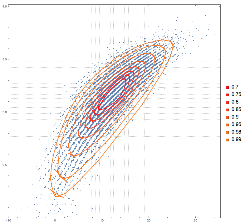
Let us similar calculations for the dataset pdData.

In[647]:= qs = {0.7, 0.75, 0.8, 0.85, 0.90, 0.95, 0.98, 0.99} ;
AbsoluteTiming[qsPoints = QuantileEnvelope[pdData, qs, 60];]
Out[648]= {0.154227, Null}


In[649]:= Dimensions[qsPoints]
Out[649]= {8, 60, 2}

Here is the plot of the dataset pdData and directional quantile envelopes.

Some more quantile curves

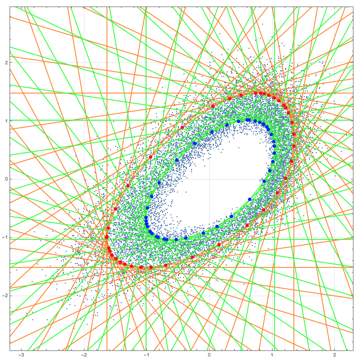
Here are couple of more plots of the quantile lines at different directions with a larger number of directions.

Lines for quantile 0.95 in 40 directions:

Lines for quantiles 0.95 and 0.8 in 40 directions:

References

[1] Anton Antonov, Quantile regression Mathematica package, source code at GitHub, https://github.com/antononcube/MathematicaForPrediction, package QuantileRegression.m, (2013).

[2] Anton Antonov, Quantile regression through linear programming, usage guide at GitHub, https://github.com/antononcube/MathematicaForPrediction, in the directory “Documentation”, (2013).

[3] Anton Antonov, Quantile regression through linear programming, “Mathematica for prediction algorithms” blog at WordPress.com, 12/16/2013.

[4] Anton Antonov, Quantile regression with B-splines, “Mathematica for prediction algorithms” blog at WordPress.com, 1/1/2014.

[5] Linglong Kong, Ivan Mizera, “Quantile tomography: using quantiles with multivariate data”, 2013, arXiv:0805.0056v2 [stat.ME] URL: http://arxiv.org/abs/0805.0056 .