Classification of handwritten digits

In this blog post I show some experiments with algorithmic recognition of images of handwritten digits.

I followed the algorithm described in Chapter 10 of the book “Matrix Methods in Data Mining and Pattern Recognition” by Lars Elden.

The algorithm described uses the so called thin Singular Value Decomposition (SVD).

1. Training phase
   1.1. Rasterize each training image into an array of 16 x 16 pixels.
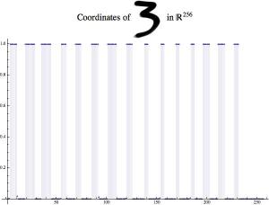
   1.2. Each raster image is linearized — the rows are aligned into a one dimensional array. In other words, each raster image is mapped into a R^256 vector space. We will call these one dimensional arrays raster vectors.
   1.3. From each set of images corresponding to a digit make a matrix with 256 columns of the corresponding raster vectors.
   1.4. Using the matrices in step 1.3 use thin SVD to derive orthogonal bases that describe the image data for each digit.

2. Recognition phase
   2.1. Given an image of an unknown digit derive its raster vector, R.
   2.2. Find the residuals of the approximations of R with each of the bases found in 1.4.
   2.3. The digit with the minimal residual is the recognition result.

The algorithm is programmed very easily with Mathematica. I did some experiments using training and test digit drawings made with the iPad app Zen Brush. I applied both the SVD recognition algorithm described above and I also applied decision trees in the same way as described in the previous blog post.

Here is a table of the training images:

And here is table of the test images:

Note that the third row is with images drawn with a thinner brush, and the fourth row is with images drawn with a thicker brush.

Here are raster images of the top row of the test drawings:

Here are several plots showing raster vectors:

      

As I mentioned earlier, raster vectors are very similar to the wave samples described in the previous blog post, so we can apply decision trees to them.

The SVD algorithm misclassified only 3 images out of 36 test digit images, success ratio 92%. Here is a table with digit drawings and list plots of the residuals:

It is interesting to look at the residuals obtained for different recognition instances. For example, the plot on the first row and first column for the recognition of a drawing of “2”  shows that the residual corresponding to 2 is the smallest and the residual for 8 is the next smallest one. The residual for 2 is the clear outlier. On the second row and third column we can see that a drawing of “4” has been classified correctly as 4, but the residual for 9 is very close to the residual for 4, we almost had a misclassification. We can see that for the other three test images with “4” the residuals for 4 are clearly separated from the rest, which can be explained with “4” being drawn more slanted, and its angle being more pronounced. Examining the misclassifications in similar way explains why they occurred.

Here are the misclassified images:

Note the misclassified image of 7 is quite different from the training images for 7.

The decision tree misclassified 42% of the images and here is are table of them:

Note that the decision trees would probably perform better if larger training data is used, not just nine drawings per digit. I also experimented with building the classifiers over the “negative” images and aligning the columns of the raster images instead of aligning the rows. The classification results were not better.

Some  details about the image preprocessing follow.

As I said, I drew the images using the Zen Brush app. For each digit I drew nine instances on Zen Brush’ canvas and exported to an image — here is an example:

Then I used Mathematica‘s function ImagePartition to partition the image into 9 singe digit drawings, and then applied ImageCrop to all them. Of course the same procedure is done for the testing images.

Further developments

Further developments with the MNIST data set are described and discussed in the blog post “Handwritten digits recognition by matrix factorization” and the forum discussion “[Mathematica-vs-R] Handwritten digits recognition by matrix factorization”.

Waveform recognition with decision trees

Few weeks ago I programmed in Mathematica the set-up of the waveform recognition problem as described in Chapter 2, Section 2.6.2 in the book “Classification And Regression Trees” by Breiman et al. Here is the document that describes the problem formulation and the classification experiments in detail: Waveform recognition with decision trees. The rest of this post is some sort of an introduction to the problem.

We have three waveforms h1, h2, h3 that are piecewise linear functions shown on this plot:

We have data array D with n rows and 21 columns. The rows of D are linear combinations of the form
 ,
in which the last term is noise generated with the normal distribution centered around 0 and standard deviation 1.

This figure shows how the rows of D look and how they can be interpreted:

The blue points represent the vectors generated with the formula above. The dashed red lines show the corresponding “clean” waves, with the noise vector ξ removed. The plot labels tell the corresponding waveform combination class labels.

The problem is:
Given D and a vector v generated with the equation above we want to determine which base waveforms have been used to generate v.

This is a classification problem, and to solve it we can construct classifiers using decision trees. Here is a short decision tree made over 300 rows of D:

As it was mentioned above, a more detailed exposition is given here: Waveform recognition with decision trees. In that document the classification problem is solved using both (i) decision trees with different tuning parameters, and (ii) random forests specific to the problem. With the random forests it is possible to attain 78-85% successful recognition. The experiments in the document also illustrate how to use the functions of the decision trees and forests package of the project MathematicaForPrediction at GitHub.

GDP per capita analysis

Let us assume that using demographic and economic data of all countries we can find correlations with high GDP per capita. In this blog post with “high GDP per capita” I mean “GDP per capita larger than $30,000.”

I used decision trees for these correlation experiments, and more specifically the implementation at the “MathematicaForPrediction” project at GitHub (https://github.com/antononcube/MathematicaForPrediction).

I built several decision trees and forests. Here is a sample of the training data:

And here it can be seen how it was labeled:

We have 176 countries labeled “low” (meaning with low GDP per capita) and 40 countries labeled “high”. (I used Mathematica‘s CountryData function.)

A great feature of decision trees is that they are easy to interpret — here is  a decision tree over the data discussed above:

Each non-leaf node of the tree has the format {impurity, splitting value, splitting variable, variable type, number of rows}. The leaf nodes are numbered, each leaf shows a label and how many countries adhere to predicate formed from the root to the leaf.

Following the edges from the root of the tree to Leaf 18 we can see that countries that have life expectancy higher that 79, birth rate fraction less than 0.014, median age higher than 33, and literacy fraction higher than 0.94 are with high GDP per capita. This rule holds for more than 50% of the countries with high GDP per capita.

Following the edges from the root of the tree to Leaf 0 we can see that countries that have life expectancy less than 74 and median age less than 33 are with low GDP per capita. This rule holds for more than 65% of the countries with low GDP per capita.

I made decision trees with more comprehensive sets of variables.  Here is a sample of the training data:

And here is the resulting decision tree: