Trie based classifiers evaluation

Posted on August 25, 2022 by Anton Antonov Antonov

Introduction

In this notebook we show how to evaluate Machine Learning (ML) classifiers based on Tries with frequencies, [AA1, AA2, AAp1], created over a well known ML dataset. The computations are done with packages and functions from the Wolfram Language (WL) ecosystem.

The classifiers based on Tries with frequencies can be seen as generalized Naive Bayesian Classifiers (NBCs).

We use the workflow summarized in this flowchart:

Import["https://raw.githubusercontent.com/antononcube/MathematicaForPrediction/master/MarkdownDocuments/Diagrams/A-monad-for-classification-workflows/Classification-workflow-horizontal-layout.jpg"]

For more details on classification workflows see the article “A monad for classification workflows”, [AA3].

Remark: This notebook is the Mathematica counterpart of the Raku computable Markdown document with the same name [AA7, AA6].

Remark: Mathematica and WL are used as synonyms in this notebook.

Data

In this section we obtain a dataset to make classification experiments with.

Through the Wolfram Function Repository (WFR) function ExampleDataset we can get data for the Titanic ship wreck:

dsTitanic0 = ResourceFunction["ExampleDataset"][{"MachineLearning", "Titanic"}];
dsTitanic0[[1 ;; 4]]

Remark: ExampleDataset uses ExampleData. Datasets from the ExampleData’s “MachineLearning” and “Statistics” collections are processed in order to obtain Dataset objects.

Instead of using the built-in Titanic data we use a version of it (which is used in Mathematica-vs-R comparisons, [AAr1]):

dsTitanic[[1 ;; 4]]

Here is a summary of the data:

ResourceFunction["RecordsSummary"][dsTitanic]

Make tries

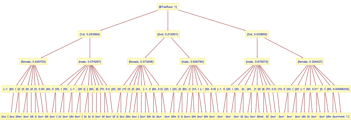
In this section for demonstration purposes let us create a shorter trie and display it in tree form.

Here we drop the identifier column and take the record fields in a particular order, in which “passengerSurvival” is the last field:

lsRecords = Normal@dsTitanic[All, Prepend[KeyDrop[#, "id"], "passengerAge" -> ToString[#passengerAge]] &][All, {"passengerClass", "passengerSex", "passengerAge", "passengerSurvival"}][Values];

Here is a sample:

RandomSample[lsRecords, 3]

(*{{"3rd", "female", "-1", "died"}, {"1st", "female", "50", "survived"}, {"3rd", "male", "30", "died"}}*)

Here make a trie without the field “passengerAge”:

trTitanic = TrieCreate[lsRecords[[All, {1, 2, 4}]]];
TrieForm[trTitanic, AspectRatio -> 1/4, ImageSize -> 900]

Here is a corresponding mosaic plot, [AA4, AAp3]:

MosaicPlot[lsRecords[[All, {1, 2, 4}]]]

Remark: The function MosaicPlot uses tries with frequencies in its implementation. Observing and reasoning with mosaic plots should make it clear that tries with frequencies are (some sort of) generalized Naive Bayesian classifiers.

Trie classifier

In this section we create a Trie-based classifier.

In order to make certain reproducibility statements for the kind of experiments shown here, we use random seeding (with SeedRandom) before any computations that use pseudo-random numbers. Meaning, one would expect WL code that starts with a SeedRandom statement (e.g. SeedRandom[89]) to produce the same pseudo random numbers if it is executed multiple times (without changing it.)

SeedRandom[12];

Here we split the data into training and testing data in a stratified manner (a split for each label):

aSplit1 = GroupBy[lsRecords, #[[-1]] &, AssociationThread[{"training", "testing"}, TakeDrop[RandomSample[#], Round[0.75*Length[#]]]] &];
Map[Length, aSplit1, {2}]

(*<|"survived" -> <|"training" -> 375, "testing" -> 125|>, "died" -> <|"training" -> 607, "testing" -> 202|>|>*)

Here we aggregate training and testing data (and show the corresponding sizes):

aSplit2 = <|
    "training" -> Join @@ Map[#training &, aSplit1], 
    "testing" -> Join @@ Map[#testing &, aSplit1]|>;
Length /@ aSplit2

(*<|"training" -> 982, "testing" -> 327|>*)

Here we make a trie with the training data (and show the node counts):

trTitanic = TrieNodeProbabilities[TrieCreate[aSplit2["training"]]];
TrieNodeCounts[trTitanic]

(*<|"total" -> 142, "internal" -> 60, "leaves" -> 82|>*)

Here is the trie in tree form:

Here is an example decision-classification:

TrieClassify[trTitanic, {"1st", "female"}]

(*"survived"*)

Here is an example probabilities-classification:

TrieClassify[trTitanic, {"1st", "female"}, "Probabilities"]

(*<|"survived" -> 0.962264, "died" -> 0.0377358|>*)

We want to classify across all testing data, but not all testing data-records might be present in the trie. Let us check that such testing records are few (or none):

Tally[Map[TrieKeyExistsQ[trTitanic, #] &, aSplit2["testing"]]]

(*{{True, 321}, {False, 6}}*)

Let us remove the records that cannot be classified:

lsTesting = Pick[aSplit2["testing"], Map[TrieKeyExistsQ[trTitanic, #] &, aSplit2["testing"]]];
Length[lsTesting]

(*321*)

Here we classify all testing records and show a sample of the obtained actual-predicted pairs:

lsClassRes = {Last[#], TrieClassify[trTitanic, Most[#]]} & /@ lsTesting;
RandomSample[lsClassRes, 6]

(*{{"survived", "survived"}, {"died", "survived"}, {"died", "died"}, {"survived", "survived"}, {"survived", "died"}, {"survived", "survived"}}*)

Here we cross tabulate the actual vs predicted labels using WFR’s CrossTabulate:

ResourceFunction["CrossTabulate"][lsClassRes]

The cross-tabulation results look bad because the default decision threshold is used. We get better results by selecting a decision threshold via Receiver Operating Characteristic (ROC) plots.

Trie classification with ROC plots

In this section we systematically evaluate the Trie-based classifier using the Receiver Operating Characteristic (ROC) framework.

Here we classify all testing data records. For each record:

Get probabilities association
Add to that association the actual label
Make sure the association has both survival labels

lsClassRes = Map[Join[<|"survived" -> 0, "died" -> 0, "actual" -> #[[-1]]|>, TrieClassify[trTitanic, #[[1 ;; -2]], "Probabilities"]] &, lsTesting];

Here we make a ROC record, [AA5, AAp4]:

ToROCAssociation[{"survived", "died"}, #actual & /@ lsClassRes, Map[If[#survived >= 0.5, "survived", "died"] &, lsClassRes]]

(*<|"TruePositive" -> 71, "FalsePositive" -> 14, "TrueNegative" -> 184, "FalseNegative" -> 52|>*)

Here we obtain the range of the label “survived”:

lsVals = Map[#survived &, lsClassRes];
MinMax[lsVals]

(*{0, 1.}*)

Here we make list of decision thresholds:

In the following code cell for each threshold:

For each classification association decide on “survived” if the corresponding value is greater or equal to the threshold
Make threshold’s ROC-association

lsROCs = Table[
    ToROCAssociation[{"survived", "died"}, #actual & /@ lsClassRes, Map[If[#survived >= th, "survived", "died"] &, lsClassRes]], 
    {th, lsThresholds}];

Here is the obtained ROCs dataset:

Dataset[MapThread[Prepend[#1, "Threshold" -> #2] &, {lsROCs, lsThresholds}]]

Here is the corresponding ROC plot:

ROCPlot["FPR", "TPR", lsThresholds, lsROCs, GridLines -> Automatic, ImageSize -> Large]

We can see the Trie-based classifier has reasonable prediction abilities – we get ≈ 80% True Positive Rate (TPR) for a relatively small False Positive Rate (FPR), ≈ 20%.

Confusion matrices

Using ClassifierMeasurements we can produce the corresponding confusion matrix plots (using “made on the spot” Manipulate interface):

DynamicModule[{lsThresholds = lsThresholds, lsClassRes = lsClassRes, lsClassRes2}, 
  Manipulate[
   lsClassRes2 = Map[{#actual, If[#survived >= lsThresholds[[i]], "survived", "died"]} &, lsClassRes]; 
   Append[DeleteCases[ClassifierMeasurements[lsClassRes2[[All, 1]], lsClassRes2[[All, 2]], "ConfusionMatrixPlot"], ImageSize -> _], ImageSize -> Medium], 
   {{i, Flatten[Position[lsThresholds, Nearest[lsThresholds, 0.3][[1]]]][[1]], "index:"}, 1, Length[lsThresholds], 1, Appearance -> "Open"}, 
   {{normalizeQ, False, "normalize?:"}, {False, True}} 
  ] 
 ]

References

Setup

Import["https://raw.githubusercontent.com/antononcube/MathematicaForPrediction/master/TriesWithFrequencies.m"];
Import["https://raw.githubusercontent.com/antononcube/MathematicaForPrediction/master/ROCFunctions.m"];
Import["https://raw.githubusercontent.com/antononcube/MathematicaForPrediction/master/MosaicPlot.m"];

dsTitanic = Import["https://raw.githubusercontent.com/antononcube/MathematicaVsR/master/Data/MathematicaVsR-Data-Titanic.csv", "Dataset", HeaderLines -> 1];

Importance of variables investigation

Posted on January 11, 2016 by Anton Antonov Antonov

Introduction

This blog post demonstrates a procedure for variable importance investigation of mixed categorical and numerical data.

The procedure was used in a previous blog “Classification and association rules for census income data”, [1]. It is implemented in the package VariableImportanceByClassifiers.m, [2], and described below; I took it from [5].

The document “Importance of variables investigation guide”, [3], has much more extensive descriptions, explanations, and code for importance of variables investigation using classifiers, Mosaic plots, Decision trees, Association rules, and Dimension reduction.

At community.wolfram.com I published the discussion opening of “Classifier agnostic procedure for finding the importance of variables” that has an exposition that parallels this blog post, but uses a different data set (“Mushroom”). (The discussion was/is also featured in “Staff picks”; it is easier to follow the Mathematica code in it.)

Procedure outline

Here we describe the procedure used (that is also done in [3]).

1. Split the data into training and testing datasets.

2. Build a classifier with the training set.

3. Verify using the test set that good classification results are obtained. Find the baseline accuracy.

4. If the number of variables (attributes) is k for each i, 1≤i≤k:

4.1. Shuffle the values of the i-th column of the test data and find the classification success rates.

5. Compare the obtained k classification success rates between each other and with the success rates obtained by the un-shuffled test data.

The variables for which the classification success rates are the worst are the most decisive.

Note that instead of using the overall baseline accuracy we can make the comparison over the accuracies for selected, more important class labels. (See the examples below.)

The procedure is classifier agnostic. With certain classifiers, Naive Bayesian classifiers and Decision trees, the importance of variables can be directly concluded from their structure obtained after training.

The procedure can be enhanced by using dimension reduction before building the classifiers. (See [3] for an outline.)

Implementation description

The implementation of the procedure is straightforward in Mathematica — see the package VariableImportanceByClassifiers.m, [2].

The package can be imported with the command:

Import["https://raw.githubusercontent.com/antononcube/MathematicaForPrediction/master/VariableImportanceByClassifiers.m"]

At this point the package has only one function, AccuracyByVariableShuffling, that takes as arguments a ClassifierFunction object, a dataset, optional variable names, and the option “FScoreLabels” that allows the use of accuracies over a custom list of class labels instead of overall baseline accuracy.

Here is the function signature:

AccuracyByVariableShuffling[ clFunc_ClassifierFunction, testData_, variableNames_:Automatic, opts:OptionsPattern[] ]

The returned result is an Association structure that contains the baseline accuracy and the accuracies corresponding to the shuffled versions of the dataset. I.e. steps 3 and 4 of the procedure are performed by AccuracyByVariableShuffling. Returning the result in the form Association[___] means we can treat the result as a list with named elements similar to the list structures in Lua and R.

For the examples in the next section we also going to use the package MosaicPlot.m, [4], that can be imported with the following command:

Import["https://raw.githubusercontent.com/antononcube/MathematicaForPrediction/master/MosaicPlot.m"]

Concrete application over the “Titanic” dataset

1. Load some data.

testSetName = "Titanic"; trainingSet = ExampleData[{"MachineLearning", testSetName}, "TrainingData"]; testSet = ExampleData[{"MachineLearning", testSetName}, "TestData"];

2. Variable names and unique class labels.

varNames = Flatten[List @@ ExampleData[{"MachineLearning", testSetName}, "VariableDescriptions"]]

(*Out[1055]= {"passenger class", "passenger age", "passenger sex", "passenger survival"} *)

classLabels = Union[ExampleData[{"MachineLearning", testSetName}, "Data"][[All, -1]]]

(*Out[1056]= {"died", "survived"} *)

3. Here is a data summary.

Grid[List@RecordsSummary[(Flatten /@ (List @@@ Join[trainingSet, testSet])) /. _Missing -> 0, varNames], Dividers -> All, Alignment -> {Left, Top}]

4. Make the classifier.

clFunc = Classify[trainingSet, Method -> "RandomForest"]

(*Out[1010]= ClassifierFunction[\[Ellipsis]] *)

5. Obtain accuracies after shuffling.

accs = AccuracyByVariableShuffling[clFunc, testSet, varNames]

(*Out[1011]= <|None -> 0.78117, "passenger class" -> 0.704835, "passenger age" -> 0.768448, "passenger sex" -> 0.610687|>*)

6. Tabulate the results.

Grid[ Prepend[ List @@@ Normal[accs/First[accs]], Style[#, Bold, Blue, FontFamily -> "Times"] & /@ {"shuffled variable", "accuracy ratio"}], Alignment -> Left, Dividers -> All]

7. Further confirmation of the found variable importance can be done using the mosaic plots.
We can see that female passengers are much more likely to survive and especially female passengers from first and second class.

t = (Flatten /@ (List @@@ trainingSet)); MosaicPlot[t[[All, {1, 3, 4}]], ColorRules -> {3 -> ColorData[7, "ColorList"]} ]

5a. In order to use F-scores instead of overall accuracy the desired class labels are specified with the option “FScoreLabels”.

accs = AccuracyByVariableShuffling[clFunc, testSet, varNames, "FScoreLabels" -> classLabels]

(*Out[1101]= <| None -> {0.838346, 0.661417}, "passenger class" -> {0.79927, 0.537815}, "passenger age" -> {0.828996, 0.629032}, "passenger sex" -> {0.703499, 0.337449}|>*)

5b. Here is another example that uses the class label with the smallest F-score.
(Probably the most important since it is most mis-classified).

accs = AccuracyByVariableShuffling[clFunc, testSet, varNames, "FScoreLabels" -> Position[#, Min[#]][[1, 1, 1]] &@ ClassifierMeasurements[clFunc, testSet, "FScore"]]

(*Out[1102]= {0.661417}, "passenger class" -> {0.520325}, "passenger age" -> {0.623482}, "passenger sex" -> {0.367521}|>*)

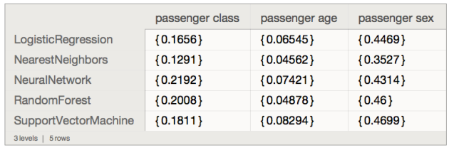
5c. It is good idea to verify that we get the same results using different classifiers. Below is given code that computes the shuffled accuracies and returns the relative damage scores for a set of methods of Classify.

mres = Association@Map[ Function[{clMethod}, cf = Classify[titanicTrainingData, Method -> clMethod]; accRes = AccuracyByVariableShuffling[cf, testSet, varNames, "FScoreLabels" -> "survived"]; clMethod -> (accRes[None] - Rest[accRes])/accRes[None] ], {"LogisticRegression", "NearestNeighbors", "NeuralNetwork", "RandomForest", "SupportVectorMachine"}] ; Dataset[mres]

References

[1] Anton Antonov, “Classification and association rules for census income data”, (2014), MathematicaForPrediction at WordPress.com.

[2] Anton Antonov, Variable importance determination by classifiers implementation in Mathematica, (2015), source code at MathematicaForPrediction at GitHub, package VariableImportanceByClassifiers.m.

[3] Anton Antonov, “Importance of variables investigation guide”, (2016), MathematicaForPrediction at GitHub, folder Documentation.

[4] Anton Antonov, Mosaic plot for data visualization implementation in Mathematica, (2014), MathematicaForPrediction at GitHub, package MosaicPlot.m.

[5] Leo Breiman et al., Classification and regression trees, Chapman & Hall, 1984, ISBN-13: 978-0412048418.

Generation of Naive Bayesian Classifiers

Posted on October 18, 2013 by Anton Antonov Antonov

This blog post is to discuss the generation of Naive Bayesian Classifiers (NBC’s) and how they can be used to explain the correlations. For more theoretical details and the Mathematica code to generate the data tables and plot in this blog post see the document “Basic theory and construction of naive Bayesian classifiers” provided by the project Mathematica For Prediction at GitHub. (The code for NBC generation and classification is also provided by that project.)

We consider the following classification problem: from a given two dimensional array representing a list of observations and labels associated with them predict the label of new, unseen observation.

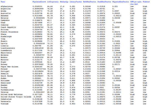
Consider for example this sample of a data array with country data:

We assume that have the following observed variables:

{“PopulationGrowth”, “LifeExpectancy”, “MedianAge”, “LiteracyFraction”, “BirthRateFraction”, “DeathRateFraction”, “MigrationRateFraction”}

The predicated variable is “GDB per capita”, the last column with the labels “high” and “low”.

Note that the values of the predicted variable “high” and “low” can be replaced with True and False respectively.

One way to solve this classification problem is to construct a NBC, and then apply that NBC to new, unknown records comprised by the observed variables.

Consider the following experiment:
1. Make a data array by querying CountryData for the observed variables
{“PopulationGrowth”, “LifeExpectancy”, “MedianAge”, “LiteracyFraction”, “BirthRateFraction”, “DeathRateFraction”, “MigrationRateFraction”, “Population”, “GDP”}

2. Replace the last two columns in the data array with a column of the labels “high” and “low”. The countries with GDP per capita greater than $30000 are labeled with “high”, the rest are labeled with “low”.

3. Split the data into a training and a testing sets.
3.1. For the training set randomly take 80% of the records with the label “high” and 80% of the records with the label “low”.
3.2. The rest of the records make the testing set.

4. Generate a NBC classifier using the training set.

5. Classify the records in the testing set with the classifier obtained at step 4.

6. Compare the actual labels with the predicted labels.
6.1. Make the comparison for all records,
6.2. only for the records labeled with “high”, and
6.3. only for the records labeled with “low”.

7. Repeat steps 3, 4, 5, and 6 if desired.

After the application of the NBC classifier implementations from the package NaiveBayesianClassifier.m we get the following predictions:

Here are the classification ratios (from step 6):

Here are the plots of the probability functions of classifier:

(Well, actually I skipped the last one for aesthetic purposes, see the document mentioned at the beginning of the blog post for all of the plots and theoretical details.)

If we imagine the Cartesian product of the probability plots we can get an idea of what kind of countries would have high GDP per capita. (I.e. more than $30000.)

	Notebook transformat… on LLM помогает в обработке перво…
	Heatmap plots over L… on Extracting Russian casualties…
	Generalized Lanchest… on A monad for Epidemiologic Comp…
	Anton Antonov Antono… on AI vision via Wolfram Lan…
	Anton Antonov Antono… on Nightcore “Conflict…

Mathematica for prediction algorithms

Using Mathematica implementations of machine learning algorithms

Category Archives: Naive Bayesian Classifier

Trie based classifiers evaluation

Introduction

Data

Make tries

Trie classifier

Trie classification with ROC plots

Confusion matrices

References

Articles

Packages

Repositories

Setup

Importance of variables investigation

Introduction

Procedure outline

Implementation description

Concrete application over the “Titanic” dataset

References

Generation of Naive Bayesian Classifiers