Classification and association rules for census income data

Introduction

In this blog post I am going to show (some) analysis of census income data — the so called “Adult” data set, [1] — using three types of algorithms: decision tree classification, naive Bayesian classification, and association rules learning. Mathematica packages for all three algorithms can be found at the project MathematicaForPrediction hosted at GitHub, [2,3,4].

(The census income data set is also used in the description of the R package “arules”, [7].)

In the census data every record represents a person with 14 attributes, the last element of a record is one of the labels {“>=50K”,”<50K”}. The relationships between the categorical variables in that data set was described in my previous blog post, “Mosaic plots for data visualization”.

For this data the questions I am most interested in are:
Question 1: Which of the variables (age, occupation, sex, etc.) are most decisive for determining the income of a person?
Question 2: Which values for which variables form conditions that would imply high income or low income? (I.e. “>50K” or “<=50K”.)
Question 3: What conclusions or confirmations we can get from answering the previous two questions?

One way to answer Question 1 is to use following steps, [8].
1. Build a classifier with the training set.
2. Verify using the test set that good classification results are obtained.
3. If the number of variables (attributes) is k for each i, 1<=i<=k :
3.1. Shuffle the values of the i-th column of the test data and find the classification success rates.
4. Compare the obtained k classification success rates between each other and with the success rates obtained by the un-shuffled test data.
5. The variables for which the classification success rates are the worst are the most decisive.

Following these steps with a decision tree classifier, [2], I found that “marital-status” and “education-num” (years of education) are most decisive to give good prediction for the “>50K” label. Using a naive Bayesian classifier, [3], the most significant variables are “marital-status” and “relationship”. (More details are given in the sections “Application of decision trees” and “Application of naive Bayesian classifier”.)

One way to answer Question 2 is to find which values of the variables (e.g. “Wife”, “Peru”, “HS-grad”, “Exec-managerial”) associate most frequently with “>50K” and “<=50K” respectively and apply different Bayesian probability statistics on them. This is what the application of Associative rules learning gives, [9]. Another way is to use mosaic plots, [5,9], and prefix trees (also known as “tries”) [6,11,12].

In order to apply Association rule learning we need to make the numerical variables categorical — we need to partition them into non-overlapping intervals. (This derived, “all categorical” data is also amenable to be input data for mosaic plots and prefix trees.)

Insights about the data set using Mosaic Plots can be found in my previous blog post “Mosaic plots for data visualization”, [13]. The use of Mosaic Plots in [13] is very similar to the Naive Bayesian Classifiers application discussed below.

Data set

The data set can be found and taken from http://archive.ics.uci.edu/ml/datasets/Census+Income, [1].

The description of the data set is given in the file “adult.names” of the data folder. The data folder provides two sets with the same type of data “adult.data” and “adult.test”; the former is used for training, the latter for testing.

The total number of records in the file “adult.data” is 32561; the total number of records in the file “adult.test” is 16281.

Here is how the data looks like:

Since I did not understand the meaning of the column “fnlwgt” I dropped it from the data.

Here is a summary of the data:

As it was mentioned in the introduction, only 24% of the labels are “>50K”. Also note that 2/3 of the records are for males.

Scatter plots and mosaic plots

Often scatter plots and mosaic plots can give a good idea of the general patterns that hold in the data. This sub-section has a couple of examples, but presenting extensive plots is beyond the scope of this blog post. Let me point out that it might be very beneficial to use these kind of plots with Mathematica‘s dynamic features (like Manipulate and Tooltip), or make a grid of mosaic plots.

Mosaic plots of the categorical variables of the data can be seen in my previous blog post “Mosaic plots for data visualization”.

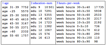
Here is a table of the histograms for “age”, “education-num”, and “hours-per-week”:

Here is a table with scatter plots for all numerical variables of the data:

Application of decision trees

The building and classification with decision trees is straightforward. Since the label “>50K” is only a quarter of the records I consider the classification success rates for “>50K” to be more important.

I experimented with several sets of parameters for decision tree building. I did not get a classification success rate for “>50K” better than 0.644 . Using pruning based on the Minimal Description Length (MDL) principle did not give better results. (I have to say I find MDL pruning to be an elegant idea, but I am not convinced that it works that
well. I believe decision tree pruning based on test data would produce much better results. Only the MDL decision tree pruning is implemented in [2].)

The overall classification success rate is in line with the classification success ratios listed in explanation of the data set; see the file “adult.names” in [1].

Here is a table with the results of the column shuffling experiments described in the introduction (in red is the name of the data column shuffled):

Here is a plot of the “>50K” success rates from the table above:

We can see from the table and the plot that variables “marital-status”, “education-num”, “capital-gain”, “age”, and “occupation” are very decisive when it comes to determining high income. The variable “marital-status” is significantly more decisive than the others.

While considering the decisiveness of the variable “marital-status” we can bring the following questions:
1. Do people find higher paying jobs after they get married?
2. Are people with high paying jobs more likely to marry and stay married?

Both questions are probably answered with “Yes” and probably that is why “marital-status” is so decisive. It is hard to give quantified answers to these questions just using decision trees on this data — we would need to know the salary and marital status history of the individuals (different data) or to be able to imply it (different algorithm).

We can see the decisiveness of “age”, “education-num”, “occupation”, and “hours-per-week” as natural. Of course one is expected to receive a higher pay if he has studied longer, has a high paying occupation, is older (more experienced), and works more hours per week. Note that this statement explicitly states the direction of the correlation: we do assume that longer years of study bring higher pay. It is certainly a good idea to consider the alternative direction of the correlation, that people first get high paying jobs and that these high paying jobs allow them to get older and study longer.

Application of naive Bayesian classifiers

The naive Bayesian classifier, [3], produced better classification results than the decision trees for the label “>50K”:

Here is a table with the results of the column shuffling experiments described in the introduction (in red is the name of the data column shuffled):

Here is a plot of the “>50K” success rates from the table above:

In comparison with the decision tree importance of variables experiments we can notice that:
1. “marital-status” is very decisive and it is the second most decisive variable;
2. the most decisive variable is “relationship” but it correlates with “marital-status”;
3. “age”, “occupation”, “hours-per-week”, “capital-gain”, and “sex” are decisive.

Shuffled classification rates plots comparison

Here are the two shuffled classification rates plots stacked together for easier comparison:

Data modification

In order to apply the association rules finding algorithm Apriori, [4], the data set have to be modified. The modification is to change the numerical variables “age”, “education-num”, and “age” into categorical. I just partitioned them into non-overlapping intervals, labeled the intervals, and assigned the labels according the variable values. Here is the summary of the modified data for just these variables:

Finding association rules

Using the modified data I found a large number of association rules with the Apriori algorithm, [4]. I used the measure called “confidence” to extract the most significant rules. The confidence of an association rule A→C with antecedent A and consequent C is defined to be the ratio P(A ∩ C)/P(C). The higher the ratio the more confidence we have in the rule. (If the ratio is 1 we have a logical rule, C ⊂ A.)

Here is a table showing the rules with highest confidence for the consequent being “>50K”:

From the table we can see for example that 2.1% of the data records (or 693 records) show that for a married man who has studied 14 years and originally from USA there is a 0.79 probability that he earns more than $50000.

Here is a table showing the rules with highest confidence for the consequent being “<=50K”:

The association rules in these tables confirm the findings with the classifiers: marital status, age, and education are good predictors of income labels “>50K” and “<=50K”.

Conclusion

The analysis confirmed (and quantified) what is considered common sense:

Age, education, occupation, and marital status (or relationship kind) are good for predicting income (above a certain threshold).

Using the association rules we see for example that
(1) if a person earns more than $50000 he is very likely to be a married man with large number of years of education;
(2) single parents, younger than 25 years, who studied less than 10 years, and were never-married make less than $50000.

References

[1] Bache, K. & Lichman, M. (2013). UCI Machine Learning Repository [http://archive.ics.uci.edu/ml]. Irvine, CA: University of California, School of Information and Computer Science. Census Income Data Set, URL: http://archive.ics.uci.edu/ml/datasets/Census+Income .

[2] Antonov, A., Decision tree and random forest implementations in Mathematica, source code at https://github.com/antononcube/MathematicaForPrediction, package AVCDecisionTreeForest.m, (2013).

[3] Antonov, A., Implementation of naive Bayesian classifier generation in Mathematica, source code at GitHub, https://github.com/antononcube/MathematicaForPrediction, package NaiveBayesianClassifier.m, (2013).

[4] Antonov, A., Implementation of the Apriori algorithm in Mathematica, source code at https://github.com/antononcube/MathematicaForPrediction, package AprioriAlgorithm.m, (2013).

[5] Antonov, A., Mosaic plot for data visualization implementation in Mathematica, source code at GitHub, https://github.com/antononcube/MathematicaForPrediction, package MosaicPlot.m, (2014).

[6] Antonov, A., Tries with frequencies Mathematica package, source code at GitHub, https://github.com/antononcube/MathematicaForPrediction, package TriesWithFrequencies.m, (2013).

[7] Hahsler, M. et al., Introduction to arules [Dash] A computational environment for mining association rules and frequent item sets, (2012).

[8] Breiman, L. et al., Classification and regression trees, Chapman & Hall, 1984.

[9] Wikipedia, Association rules learning, http://en.wikipedia.org/wiki/Association_rule_learning .

[10] Antonov, A., Mosaic plots for data visualization, (March, 2014), MathematicaForPrediction at GitHub, URL: https://github.com/antononcube/MathematicaForPrediction/blob/master/Documentation/Mosaic%20plots%20for%20data%20visualization.pdf .

[11] Wikipedia, Trie, http://en.wikipedia.org/wiki/Trie .

[12] Antonov, A., Tries, (December, 2013), URL: https://github.com/antononcube/MathematicaForPrediction/blob/master/Documentation/Tries.pdf .

[13] Antonov, A., Mosaic plots for data visualization, (March, 2014) MathematicaForPrediction at WordPress.