Generation of Naive Bayesian Classifiers

This blog post is to discuss the generation of Naive Bayesian Classifiers (NBC’s) and how they can be used to explain the correlations. For more theoretical details and the Mathematica code to generate the data tables and plot in this blog post see the document “Basic theory and construction of naive Bayesian classifiers” provided by the project Mathematica For Prediction at GitHub. (The code for NBC generation and classification is also provided by that project.)

We consider the following classification problem: from a given two dimensional array representing a list of observations and labels associated with them predict the label of new, unseen observation.

Consider for example this sample of a data array with country data:
CountryData data array sample

We assume that have the following observed variables:

{“PopulationGrowth”, “LifeExpectancy”, “MedianAge”, “LiteracyFraction”, “BirthRateFraction”, “DeathRateFraction”, “MigrationRateFraction”}

The predicated variable is “GDB per capita”, the last column with the labels “high” and “low”.

Note that the values of the predicted variable “high” and “low” can be replaced with True and False respectively.

One way to solve this classification problem is to construct a NBC, and then apply that NBC to new, unknown records comprised by the observed variables.

Consider the following experiment:
1. Make a data array by querying CountryData for the observed variables
{“PopulationGrowth”, “LifeExpectancy”, “MedianAge”, “LiteracyFraction”, “BirthRateFraction”, “DeathRateFraction”, “MigrationRateFraction”, “Population”, “GDP”}

2. Replace the last two columns in the data array with a column of the labels “high” and “low”. The countries with GDP per capita greater than $30000 are labeled with “high”, the rest are labeled with “low”.

3. Split the data into a training and a testing sets.
3.1. For the training set randomly take 80% of the records with the label “high” and 80% of the records with the label “low”.
3.2. The rest of the records make the testing set.

4. Generate a NBC classifier using the training set.

5. Classify the records in the testing set with the classifier obtained at step 4.

6. Compare the actual labels with the predicted labels.
6.1. Make the comparison for all records,
6.2. only for the records labeled with “high”, and
6.3. only for the records labeled with “low”.

7. Repeat steps 3, 4, 5, and 6 if desired.

After the application of the NBC classifier implementations from the package NaiveBayesianClassifier.m we get the following predictions:
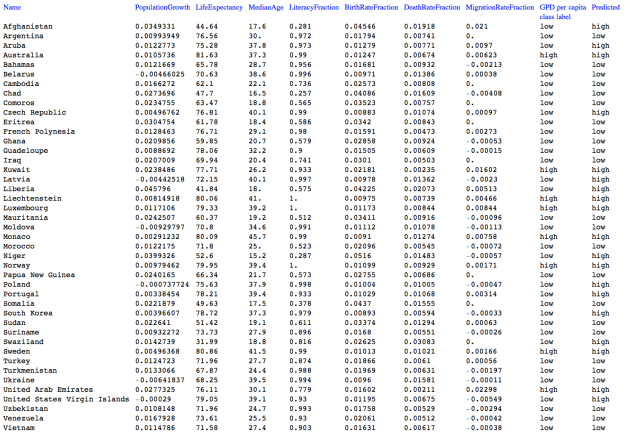
CountryData test records with actual and predicted labels
Here are the classification ratios (from step 6):
Success ratios

Here are the plots of the probability functions of classifier:
Probability functions for country data variables

(Well, actually I skipped the last one for aesthetic purposes, see the document mentioned at the beginning of the blog post for all of the plots and theoretical details.)

If we imagine the Cartesian product of the probability plots we can get an idea of what kind of countries would have high GDP per capita. (I.e. more than $30000.)

Outlier detection in a list of numbers

Introduction

I added today a Mathematica package with outlier detection algorithms in the project MathematicaForPrediction at GitHub. I also wrote and uploaded a guide to using the functions in this package — see “Outlier detection in a list of numbers“.

I frequently include outlier identification in the interfaces and algorithms I make for search and prediction engines. Of course, outlier identification is also indispensable for data cleaning, normalization, and analysis.

My first introduction to outlier detection was through the book “Mining Imperfect Data: Dealing with Contamination and Incomplete Records” by Ronald K. Pearson. (Here is also a link to that book at amazon.com.)

Outlier detection basics

The purpose of the outlier detection algorithms is to find those elements in a list of numbers that have values significantly higher or lower than the rest of the values.

Taking a certain number of elements with the highest values is not the same as an outlier detection, but it can be used as a replacement.

Let us consider the following set of 50 numbers:

pnts = RandomVariate[GammaDistribution[5, 1], 50]

(* {7.59113, 5.57539, 3.77879, 3.14141, 5.25833, 7.4036, 5.7324, 4.3612, \
3.04052, 4.30872, 7.79725, 8.12759, 6.75185, 4.39845, 8.12002, \
2.95435, 9.55785, 4.06057, 3.27145, 10.2521, 3.52952, 6.25076, \
1.82362, 2.8844, 4.22082, 1.94356, 2.39944, 3.97935, 6.11422, \
4.80236, 8.56683, 3.61667, 2.53776, 3.60869, 2.56662, 4.05317, \
2.27279, 4.46844, 4.57981, 5.00396, 4.17491, 10.4406, 4.31504, \
4.83232, 4.56361, 5.38989, 2.66085, 2.37754, 3.21949, 3.53067} *)

If we sort those numbers descendingly and plot them we get:

pnts = pnts // Sort // Reverse;
ListPlot[pnts, PlotStyle -> {PointSize[0.015]}, Filling -> Axis, PlotRange -> All]

ListPlotOfSorted50Numbers

Let us use the following outlier detection algorithm:
1. find all values in the list that are larger than the mean value multiplied by 1.5;
2. then find the positions of these values in the list of numbers.

We can implement this algorithm in the following way.

pos = Flatten[Map[Position[pnts, #] &, Select[pnts, # > 1.5 Mean[pnts] &]]]

(* {1, 2, 3, 4, 5, 6, 7, 8, 9} *)

Lets plot all points in blue and the outliers we found in red:

ListPlot[{pnts, Transpose[{pos, pnts[[pos]]}]}, 
 PlotStyle -> {PointSize[0.015], PointSize[0.009]}, Filling -> Axis, 
 PlotRange -> All]

ListPlotOfSorted50NumbersWithOutliers

Instead of the mean value we can use another reference point, like the median value. Obviously, we can also use a multiplier different than 1.5.

Using the implementation

First let us load the outlier identification package:

Get["https://github.com/antononcube/MathematicaForPrediction/blob/master/OutlierIdentifiers.m"]

We can find the outliers in a list of numbers with the function OutlierIdentifier:

OutlierIdentifier[pnts, HampelIdentifierParameters]

(* {10.4406, 10.2521, 9.55785, 8.56683, 8.12759, 8.12002, 7.79725, 7.59113, \
7.4036, 6.75185, 6.25076, 2.39944, 2.37754, 2.27279, 1.94356, 1.82362} *)

The package has three functions for the calculation of outlier identifier parameters over a list of numbers

HampelIdentifierParameters[pnts]
(* {2.50757, 6.11619} *)

SPLUSQuartileIdentifierParameters[pnts]
(* {-0.549889, 9.50178} *)

QuartileIdentifierParameters[pnts]
(* {1.79581, 6.82164} *)

Elements of the number list that are outside of the numerical interval made by one of these pairs of numbers are considered outliers.

In many cases we want only the top outliers or only the bottom outliers. We can use the functions TopOutliers and BottomOutliers for that.

OutlierIdentifier[pnts, TopOutliers[HampelIdentifierParameters[#]] &]

(* {10.4406, 10.2521, 9.55785, 8.56683, 8.12759, 8.12002, 7.79725, 7.59113, 7.4036, 6.75185, 6.25076} *)

Statistical thesaurus from NPR podcasts

Five months ago I worked with transcripts of National Public Radio (NPR) podcasts. The transcripts are available at http://www.npr.org — see for example “From child actor to artist…“.

Using nearly 5000 transcripts I experimented with topic extraction and statistical thesaurus derivation. The topics are too bulky to show here, but I am going to show some of the statistical thesaurus entries.

I used dimension reduction with Non-Negative Matrix Factorization (NNMF). For more detailed explanations, code for computations, and experimental results see this paper “Topic and thesaurus extraction from a document collection” provided by the MathematicaForPrediction project at GitHub. (The code for NNMF is also provided by the MathematicaForPrediction project at GitHub.)

First let me describe the data. The collection has 5123 transcripts.

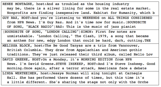
Here is a sample of the transcripts (only the first 400 characters of each are taken):
NPR podcast sample 400 characters per podcast

Here is the distribution of the string lengths of the transcripts:
5123 NPR podcasts string length

I removed custom selected stop words from the transcripts. I also stemmed the words using the stemmer called snowball, see http://snowball.tartarus.org. The stemmed words are called “terms” below.

Here are descriptive statistics and the distribution of the number of transcripts per term:
Transcripts per term

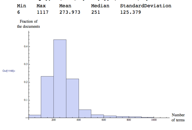
Here are descriptive statistics and the distribution of the number of terms per transcript:
Terms per transcript

I did not compute the whole statistical thesaurus. Instead I made a function that computes the thesaurus entry of a given word using the right NNMF factor with proper normalization.

Here are sample results of the thesaurus entry “retrieval” (note that the right column contains word stems):
Statistical thesaurus entries

Movie genre associations

In this post we are going to look at genre associations deduced by extracting association rules from a catalog of movies. For example, we might want to confirm that most romance movies are also dramas, and we want to find similar rules. For more details see this user guide https://github.com/antononcube/MathematicaForPrediction/blob/master/Documentation/MovieLens%20genre%20associations.pdf at Mathematica for Prediction at GitHub .

The movie data was taken from the page MovieLens Data Sets (http://www.grouplens.org/taxonomy/term/14) of the site GroupLens Research (http://www.grouplens.org). More precisely, the data set named “MovieLens 10M Data Set” was taken.

We are interested in the movie-genre relations only and if we look only at the movie-genre relations of “MovieLens 10M Data Set” the movies are poorly interconnected. Approximately 40% of the movies have only one genre. We use MovieLens since it is publicly available, easy to ingest, and the presented results can be reproduced.

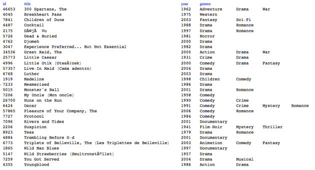
Here is a sample of the movie-genre data:
MovieLens 10k movie-genre data sample

Let us first look into some descriptive statistics of the data set.

We have 10681 movies, and 18 genres. Here is a breakdown of the movies across the genres:
MovieLens 10k movie-genre data genre breakdown

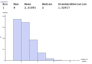
Here are a table of descriptive statistics and a histogram of the distribution of the number of genres:
MovieLens 10k Descriptive statistics for the number of genres

Here are a table of descriptive statistics and a histogram with the distribution of the movies across the release years:
MovieLens 10k Release years descriptive statistics

I applied to the movie-genre data the algorithm Apriori which is an associative rules learning algorithm. The Mathematica implementation is available at this link: https://github.com/antononcube/MathematicaForPrediction/blob/master/AprioriAlgorithm.m

With the Apriori algorithm we can find frequent association genre sets. In order to apply Apriori from each data row only the genres are taken. In this way we can see each movie as a “basket” of genres or as a “transaction” of genres, and the total movie catalog as a set of transactions.

In order to extract association rules from each frequent set we apply different measures. The GitHub package provides five measures: Support, Confidence, Lift, Leverage, and Conviction. The measure Support follows the standard mathematical definition (fraction of the total number of transactions) and it is used to find the association sets. Conviction is considered to be the best for uncovering interesting rules. The definition and interpretation of the measures are given in these tables:
Tables of definitions and properties of association rules measures

I implemented a dynamic interface to browse the association sets that have support higher than 0.25% :
Association sets dynamic interface

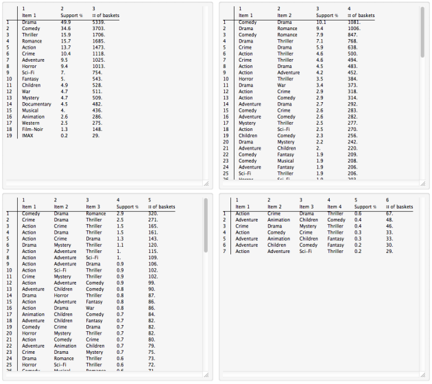
This 2×2 table of interface snapshots shows the association sets that have the largest support:
Association sets interface snapshots

We can see that — as expected — “Romance” and “Drama” are highly associated. Other expected associations are {“Comedy”, “Drama”, “Romance”} , {“Crime”, “Drama”, “Thriller”}, and {“Action”, “Crime”, “Thriller”}.

I also implemented a dynamic interface for browsing the association rules extracted from the frequent sets. Here is a list of snapshots of that interface:
1. Association rules of 2 items for all genres ordered by Conviction:
2 item rules for All ordered by Conviction
2. Association rules of 3 items for all genres ordered by Conviction:
3 item rules for All ordered by Conviction
3. Association rules of 2 items with “Drama” ordered by Conviction:
2 item rules for Drama ordered by Conviction
4. Association rules of 3 items with “Drama” ordered by Conviction:
3 item rules for Drama ordered by Conviction

Again, the results we see are expected. For example, looking at the measure Confidence we can see that for the MovieLens 10k catalog 82% of the romance-war movies are also dramas, and 73% of the war movies are dramas. In a certain sense, “War” and {“Romance”, “War”} function like sub-genres of “Drama”.