Quantile regression robustness

This blog post shows examples of quantile regression robustness. The quantile regression curves (called “regression quantiles”) are computed with the Mathematica package QuantileRegression.m hosted at the MathematicaForPrediction project at GitHub. Quantile regression was introduced by Koenker and Bassett in 1978; detailed theoretical descriptions and discussions are given in the book “Quantile regression” by Koenker.

This blog post extends the previous blog post.

Here is a scattered points graph based on a simple deterministic model with a simple heteroscedasticity (the variance varies with x):

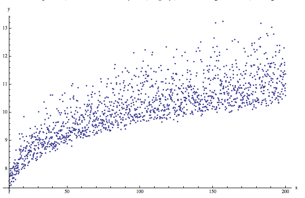
The data was generated with the Mathematica command:

{#, 5 + Log[#] + RandomReal[SkewNormalDistribution[0, Log[#]/5, 12]]} & /@ Range[10,200,0.126751]

Looking at the plot we would assume that the model for the data is

Y = β0 +β1 * X + β3 * log(X).

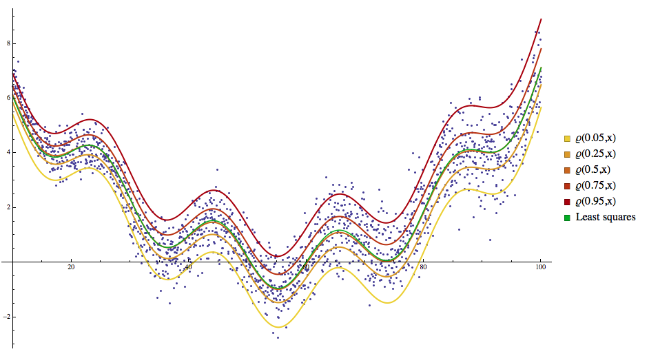
Here is a plot of the data and the regression quantiles:

Let us demonstrate the robustness of the regression quantiles with the data of the previous example. Suppose that for some reason 50% of the data y-values greater than 11.25 are altered by multiplying them with a some greater than 1 factor, say, α = 1.8 . Then the altered data looks like this:

Here is a plot of altered data and the regression quantiles and least squares fit for the altered data:

Let us pair up the old regression quantile formulas with the new ones. We can see that the new regression quantiles computed for 0.05, 0.25, and 0.5 have not changed significantly:

Also, there is a significant change in least squares fit:

(i) original data: 5.02011 + 0.000708203 x + 1.14048 Log[x],

(ii) altered dataL 6.60508 + 0.0183379 x + 0.494545 Log[x].

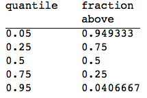
Here is a table of applying the altered regression quantiles to the original data:

Now let us do a different type of alternation of the original data. Suppose that for some reason 70 % of the data Y-values above 0.95 regression quantile are the altered by multiplying them with a some greater than 1 factor, say, α = 10 . Then the altered data looks like this (using a log-plot):

Here is a plot of the altered data and all fitted functions:

Note that the least squares fit is quite off (the plot has a logarithmic scale on the y-axis). We can see that the new regression quantiles computed for 0.05, 0.25, 0.5, 0.75, and 0.95 have not changed significantly:

Here is a table of applying the altered regression quantiles to the original data:

The examples clearly demonstrate the robustness of quantile regression when compared to the least squares fit. As in the single distribution case, computing quantiles can be very useful for identifying outliers. For example, we can do the regression analogue of standardizing the data by subtracting the median and dividing by the interquartile distances, and declare any point outside of a specified range as an outlier.

Quantile regression through linear programming

We can say that least squares linear regression corresponds to finding the mean of a single distribution. Similarly, quantile regression corresponds to finding quantiles of a single distribution. With quantile regression we obtain curves — “regression quantiles” — that together with the least squares regression curve would give a more complete picture of the distribution values (the Y’s) corresponding to a set of X’s.

The Quantile Regression Problem (QRP) is formulated as a minimization of the sum of absolute differences. Further, QRP is re-formulated as a linear programming problem, which allows for efficient computation. To compute quantiles other than the median the so called “tilted” function is used. (See this Wikipedia entry.)

For a complete, interesting, and colorful introduction and justification to quantile regression I refer to this article:

Roger Koenker, Gilbert Bassett Jr., “Regression Quantiles”, Econometrica, Vol. 46, No. 1. (Jan., 1978), pp. 33-50. JSTOR URL: http://links.jstor.org/sici?sici=0012-9682%28197801%2946%3A1%3C33%3ARQ%3E2.0.CO%3B2-J .

I recently implemented and uploaded a Mathematica package for computing regression quantiles using Mathematica’s function LinearProgramming — see the package QuantileRegression.m provided by the MathematicaForPrediction project at GitHub. Also see this guide for using the function QuantileRegressionFit provided by the package. The guide has some theoretical explanations and shows how the quantile regression problem can be formulated as a linear programming problem.

Below are presented several examples of regression quantiles computed over different data sets with the function QuantileRegressionFit provided by the package. The signature of QuantileRegressionFit is very similar to that of Mathematica‘s function Fit. Here is the definition statement:

QuantileRegressionFit::usage = “QuantileRegressionFit[data,funs,var,qs] finds the regression quantiles corresponding to the quantiles qs for a list of data as linear combinations of the functions funs of the variable var.”

QuantileRegressionFit has a Method option and can use both Minimize and LinearProgramming, but the computations with Minimize are quite slow for larger data sets. (The implementation with Minimize is included for didactic purposes.) All QuantileRegressionFit results presented below are done with the linear programming implementation.

First let us consider data generated by adding skewed noise over a logarithmic curve:

Pretending that we don’t know how the data is generated, just by looking at the plot, we might conjecture that the model for the data is

Y = b0 + b1 X + b2 X^(1/2) + b3 log(X) .

Using this model we find regression quantiles corresponding to 0.05, 0.25, 0.5, 0.75, 0.95. For comparison we also find the least squares fit of the model. Here is a plot that shows the regression quantiles for that data together with the least squares fit of the model functions:

We can check do the regression quantiles partition the data in the expected way. Here is a table that shows the fraction of the data points with Y’s greater or equal than the corresponding regression quantile:

Here is a plot of the with the regression quantiles of a more interesting set of data:

Here is the table for the data partition tests:

I further made some performance profiling tests. First we need to choose a family or several families of test data. Also, since Mathematica’s function LinearProgramming has several methods it is a good idea to test with all of them. Here I am going to show results only with one family of data and two LinearProgramming methods. The data family is the skewed noise over a logarithmic curve used as an example above. The first LinearProgramming method is Mathematica‘s  (default) “InteriorPoint”, the second method is “CLP” that uses the built-in COIN-OR CLP optimizer. I run the profiling tests using one quantile {0.5} and five quantiles {0.05, 0.25, 0.5, 0.75, 0.95}, which are shown in blue and red respectively. I also run tests with different number of model functions {1, x, x^(1/2), log(x)} and {1, x, log(x)} but there was no significant difference in the timings (less than 2%).

It is interesting to note that the average ratio of the timings with 1 vs. 5 quantiles is 0.38 for “InteriorPoint” and 0.5 for “CLP”.

In another post I am going to show examples of the robustness of regression quantiles when the data has outliers.

Update: Because I implemented calculation of regression quantiles with B-splines I had to rename the function QuantileRegression into QuantileRegressionFit. I made the corresponding changes in the blog post. (Except the profile graphics captions.)

Tries with frequencies for data mining

In computer science a trie (or a prefix tree) is a data structure that allows quick retrieval of associations between a set of keys and a set of values. It is assumed that each key is a sequence of elements. (Most often the keys are considered to be strings i.e. sequences of characters.) The trie nodes do not store the keys. Instead the position of a node in a trie corresponds to a key.

For example, if we have the list of words

{“war”, “ward”, “warden”, “work”, “car”, “cars”, “carbs”}

we can make the trie:

We can further shrink the trie in order to find the internal “prefixes”:

Another transformation of a trie is to replace the numbers of appearances with probabilities — each value of a node is the probability to arrive to that node from the parent:

Using this last trie we can take a Bayesian perspective and ask questions like: Given that a word starts with “ca” what is the probability the word to end with “s” or “r”? (Within the set of words we built the trie with.)

This document has an introduction to tries with frequencies and it is also a guide to using the package described below. The document has lots of examples and illustrative graph plots; it also discusses how to answer the Bayesian questions.

Several years ago I started experimenting with applying tries to data mining problems. During the last few months I productized my Mathematica trie implementations into a package — see the package TriesWithFrequencies.m provided by the MathematicaForPrediction project at GitHub. The package is for creation, manipulation, and visualization of tries in which the key values are frequencies of appearance in the data that is data mined. The package can also be used to build and use tries as associative arrays.

Using tries for data mining comes from the general idea of utilizing NLP techniques and algorithms in non-language problems. Such an utilization is possible because, philosophically speaking, in the current Big Data + Facebook phase of our civilization every entity can be, and it is, characterzied with tags. If we have a collection of events and they are tagged properly with a good system of tags we can data mine sequences of events with prefix trees.