Maze making using graphs

Introduction

This document (notebook) describes three ways of making mazes (or labyrinths) using graphs. The first two are based on rectangular grids; the third on a hexagonal grid.

All computational graph features discussed here are provided by the Graph functionalities of Wolfram Language.

TL;DR

Just see the maze pictures below. (And try to solve the mazes.)

Procedure outline

The first maze is made by a simple procedure which is actually some sort of cheating:

  • A regular rectangular grid graph is generated with random weights associated with its edges.
  • The (minimum) spanning tree for that graph is found.
  • That tree is plotted with exaggeratedly large vertices and edges, so the graph plot looks like a maze.
    • This is “the cheat” — the maze walls are not given by the graph.

The second maze is made “properly”:

  • Two interlacing regular rectangular grid graphs are created.
  • The second one has one less row and one less column than the first.
  • The vertex coordinates of the second graph are at the centers of the rectangles of the first graph.
  • The first graph provides the maze walls; the second graph is used to make paths through the maze.
    • In other words, to create a solvable maze.
  • Again, random weights are assigned to edges of the second graph, and a minimum spanning tree is found.
  • There is a convenient formula that allows using the spanning tree edges to remove edges from the first graph.
  • In that way, a proper maze is derived.

The third maze is again made “properly” using the procedure above with two modifications:

  • Two interlacing regular grid graphs are created: one over a hexagonal grid, the other over a triangular grid.
    • The hexagonal grid graph provides the maze walls; the triangular grid graph provides the maze paths.
  • Since the formula for wall removal is hard to derive, a more robust and universal method based on nearest neighbors is used.

Simple Maze

In this section, we create a simple, “cheating” maze.

Remark: The steps are easy to follow, given the procedure outlined in the introduction.

RandomSeed[3021];
{n, m} = {10, 25};
g = GridGraph[{n, m}];
gWeighted = Graph[VertexList[g], UndirectedEdge @@@ EdgeList[g], EdgeWeight -> RandomReal[{10, 1000}, EdgeCount[g]]];
Information[gWeighted]

0s0wsdfzitdzq

Find the spanning tree of the graph:

mazeTree = FindSpanningTree[gWeighted];

Shortest path from the first vertex (bottom-left) to the last vertex (top-right):

path = FindShortestPath[mazeTree, 1, n*m];
Length[path]

Out[]= 46

Graph plot:

simpleMaze = Graph[VertexList[mazeTree], EdgeList[mazeTree], VertexCoordinates -> GraphEmbedding[g]];
 simpleMaze2 = EdgeAdd[simpleMaze, {"start" -> 1, Max[VertexList[simpleMaze]] -> "end"}];
 Clear[vf1, ef1];
 vf1[col_?ColorQ][{xc_, yc_}, name_, {w_, h_}] := {col, EdgeForm[None],Rectangle[{xc - w, yc - h}, {xc + w, yc + h}]};
 ef1[col_?ColorQ][pts_List, e_] := {col, Opacity[1], AbsoluteThickness[22], Line[pts]};
 grCheat = GraphPlot[simpleMaze2, VertexSize -> 0.8, VertexShapeFunction -> vf1[White], EdgeShapeFunction -> ef1[White], Background -> DarkBlue, ImageSize -> 800, ImagePadding -> 0];
 range = MinMax /@ Transpose[Flatten[List @@@ Cases[grCheat, _Rectangle, \[Infinity]][[All, All]], 1]];
 Show[grCheat, PlotRange -> range]

1bc8vj9fmf5ro

The “maze” above looks like a maze because the vertices and edges are rectangular with matching sizes, and they are thicker than the spaces between them. In other words, we are cheating.

To make that cheating construction clearer, let us plot the shortest path from the bottom left to the top right and color the edges in pink (salmon) and the vertices in red:

gPath = PathGraph[path, VertexCoordinates -> GraphEmbedding[g][[path]]];
Legended[
   Show[
    grCheat, 
    Graph[gPath, VertexSize -> 0.7, VertexShapeFunction -> vf1[Red], EdgeShapeFunction -> ef1[Pink], Background -> DarkBlue, ImageSize -> 800, ImagePadding -> 0], 
    PlotRange -> range 
   ], 
   SwatchLegend[{Red, Pink, DarkBlue}, {"Shortest path vertices", "Shortest path edges", "Image background"}]]

1q29onggyuwcc

Proper Maze

proper maze is a maze given with its walls (not with the space between walls).

Remark: For didactical reasons, the maze in this section is small so that the steps—outlined in the introduction—can be easily followed.

Make two regular graphs: one for the maze walls and the other for the maze paths.

{n, m} = {6, 12};
g1 = GridGraph[{n, m}, VertexLabels -> "Name"];
g1 = VertexReplace[g1, Thread[VertexList[g1] -> Map[w @@ QuotientRemainder[# - 1, n] &, VertexList[g1]]]];
g2 = GridGraph[{n - 1, m - 1}];
g2 = VertexReplace[g2, Thread[VertexList[g2] -> Map[QuotientRemainder[# - 1, n - 1] &, VertexList[g2]]]];
g2 = Graph[g2, VertexLabels -> "Name", VertexCoordinates -> Map[# + {1, 1}/2 &, GraphEmbedding[g2]]];
Grid[{{"Wall graph", "Paths graph"}, {Information[g1], Information[g2]}}]

0t91asf2eugz2

See how the graph “interlace”:

(*Show[g1,HighlightGraph[g2,g2],ImageSize->800]*)

Maze Path Graph:

mazePath = Graph[EdgeList[g2], EdgeWeight -> RandomReal[{10, 10000}, EdgeCount[g2]]];
mazePath = FindSpanningTree[mazePath, VertexCoordinates -> Thread[VertexList[g2] -> GraphEmbedding[g2]]];
Information[mazePath]

0t91asf2eugz2

Combined Graph:

g3 = Graph[
     Join[EdgeList[g1], EdgeList[mazePath]], VertexCoordinates -> Join[Thread[VertexList[g1] -> GraphEmbedding[g1]], Thread[VertexList[mazePath] -> GraphEmbedding[mazePath]]], 
     VertexLabels -> "Name"];
Information[g3]

0mdi2hih68mqo

Plot the combined graph:

HighlightGraph[g3, mazePath, ImageSize -> 800]

1kndzl5jned4z

Remove wall edges using a formula:

g4 = Graph[g3, VertexLabels -> None]; 
  
Do[{i, j} = e[[1]]; 
      {i2, j2} = e[[2]]; 
      If[i2 < i || j2 < j, {{i2, j2}, {i, j}} = {{i, j}, {i2, j2}}]; 
      
     (*Horizontal*) 
      If[i == i2 && j < j2, 
       g4 = EdgeDelete[g4, UndirectedEdge[w[i2, j2], w[i2 + 1, j2]]] 
      ]; 
      
     (*Vertical*) 
      If[j == j2 && i < i2, 
       g4 = EdgeDelete[g4, UndirectedEdge[w[i2, j2], w[i2, j2 + 1]]] 
      ]; 
     , {e, EdgeList[mazePath]}]; 
  
Information[g4]

0s9eo0feadbo8

Plot wall graph and maze paths (maze space) graph:

HighlightGraph[g4, mazePath, ImageSize -> 800]

05ekkh85mpfro

Fancier maze presentation with rectangular vertices and edges (with matching sizes):

g5 = Subgraph[g4, VertexList[g1]];
g5 = VertexDelete[g5, {w[0, 0], w[m - 1, n - 1]}];
g6 = Graph[g5, VertexShapeFunction -> None, EdgeShapeFunction -> ({Opacity[1], DarkBlue, AbsoluteThickness[30], Line[#1]} &), ImageSize -> 800]

0arq97krotgni

Here is how a solution can found and plotted:

(*solution=FindPath[#,VertexList[#][[1]],VertexList[#][[-1]]]&@mazePath;
 Show[g6,HighlightGraph[Subgraph[mazePath,solution],Subgraph[mazePath,solution]]]*)

Here is a (more challenging to solve) maze generated with $n=12$ and $m=40$:

1tmgs2lmz563k

Hexagonal Version

Let us create another maze based on a hexagonal grid. Here are two grid graphs:

  • The first is a hexagonal grid graph representing the maze’s walls.
  • The second graph is a triangular grid graph with one fewer row and column, and shifted vertex coordinates.
{n, m} = {6, 14}*2; 
g1 = ResourceFunction["HexagonalGridGraph"][{m, n}]; 
g1 = VertexReplace[g1, Thread[VertexList[g1] -> (w[#1] & ) /@ VertexList[g1]]]; 
g2 = ResourceFunction["https://www.wolframcloud.com/obj/antononcube/DeployedResources/Function/TriangularLatticeGraph/"][{n - 1, m - 1}]; 
g2 = Graph[g2, VertexCoordinates -> (#1 + {Sqrt[3], 1} & ) /@ GraphEmbedding[g2]]; 
{Information[g1], Information[g2]}

0eyicaepipiwo
Show[g1, HighlightGraph[g2, g2], ImageSize -> 800]

0bfc3uk2c4uw3

Maze Path Graph:

mazePath = Graph[EdgeList[g2], EdgeWeight -> RandomReal[{10, 10000}, EdgeCount[g2]]];
 mazePath = FindSpanningTree[mazePath, VertexCoordinates -> Thread[VertexList[g2] -> GraphEmbedding[g2]]];
 Information[mazePath]

0937puga1ahjz

Combine the walls-maze and the maze-path graphs (i.e., make a union of them), and plot the resulting graph:

g3 = GraphUnion[g1, mazePath, VertexCoordinates -> Join[Thread[VertexList[g1] -> GraphEmbedding[g1]], Thread[VertexList[mazePath] -> GraphEmbedding[mazePath]]]];
 Information[g3]

1foiaesyk9d5s
HighlightGraph[g3, mazePath, ImageSize -> 800]

1t4t24o8zwj7p

Make a nearest neighbor points finder functor:

finder = Nearest[Thread[GraphEmbedding[g1] -> VertexList[g1]]]

045ypuvgpbrq4

Take a maze edge and its vertex points:

e = First@EdgeList[mazePath];
aMazePathCoords = Association@Thread[VertexList[mazePath] -> GraphEmbedding[mazePath]];
 points = List @@ (e /. aMazePathCoords)

17k4mshnxw0tf

Find the edge’s midpoint and the nearest wall-graph vertices:

Print["Middle edge point: ", Mean[points]]
Print["Edge to remove: ", UndirectedEdge @@ finder[Mean[points]]]

0b52fvogi84bf
1xlaj83jf90c6

Loop over all maze edges, removing wall-maze edges:

g4 = g1;
Do[
    points = Map[aMazePathCoords[#] &, List @@ e]; 
     m = Mean[points]; 
     vs = finder[m]; 
     g4 = EdgeDelete[g4, UndirectedEdge @@ vs]; 
    , {e, EdgeList[mazePath]}] 
  
Information[g4]

11uvhhgtj2da4

Here is the obtained graph

Show[g4, ImageSize -> 800]

0zih3bdnlu25c

The start and end points of the maze:

aVertexCoordinates = Association@Thread[VertexList[g4] -> GraphEmbedding[g4]];
{start, end} = Keys[Sort[aVertexCoordinates]][[{1, -1}]]

Out[]= {w[1], w[752]}

Finding the Maze Solution:

Out[]= Sequence[1, 240]

solution = FindShortestPath[mazePath, Sequence @@ Keys[Sort[aMazePathCoords]][[{1, -1}]]];
solution = PathGraph[solution, VertexCoordinates -> Lookup[aMazePathCoords, solution]];

Plot the maze:

g5 = Graph[g4, VertexShapeFunction -> None, EdgeShapeFunction -> ({Opacity[1], DarkBlue, AbsoluteThickness[8], Line[#1]} &), ImageSize -> 800];
g5 = VertexDelete[g5, {start, end}]

0lpxgk7luqu30

Here is the solution of the maze:

Show[g5, HighlightGraph[solution, solution]]


Additional Comments


References

Articles, Blog Posts

[AA1] Anton Antonov, “Day 24 — Maze Making Using Graphs”, (2025), Raku Advent Calendar at WordPress .

Functions

[AAf1] Anton Antonov, TriangularLatticeGraph, (2025), Wolfram Function Repository.

[EWf1] Eric Weisstein, TriangularGridGraph, (2020), Wolfram Function Repository.

[WRIf1] Wolfram Research, HexagonalGridGraph, (2020), Wolfram Function Repository.

Packages

[AAp1] Anton Antonov, Graph, Raku package , (2024–2025), GitHub/antononcube .

[AAp2] Anton Antonov, Math::Nearest, Raku package , (2024), GitHub/antononcube .

Numerically 2026 is unremarkable yet happy

… and has primitive roots

Introduction

This document (notebook) discusses number theory properties and relationships of the integer 2026.

The integer 2026 is semiprime and a happy number, with 365 as one of its primitive roots. Although 2026 may not be particularly noteworthy in number theory, this provides a great excuse to create various elaborate visualizations that reveal some interesting aspects of the number.

Setup

(*PacletInstall[AntonAntonov/NumberTheoryUtilities]*)
   Needs["AntonAntonov`NumberTheoryUtilities`"]

2026 Is a Happy Semiprime with Primitive Roots

First, 2026 is obviously not prime—it is divisible by 2 —but dividing it by 2 gives a prime, 1013:

PrimeQ[2026/2]

Out[]= True

Hence, 2026 is a semiprime . The integer 1013 is not a Gaussian prime , though:

PrimeQ[1013, GaussianIntegers -> True]

Out[]= False

happy number is a number for which iteratively summing the squares of its digits eventually reaches 1 (e.g., 13 -> 10 -> 1). Here is a check that 2026 is happy:

ResourceFunction["HappyNumberQ"][2026]

Out[]= True

Here is the corresponding trail of digit-square sums:

FixedPointList[Total[IntegerDigits[#]^2] &, 2026]

Out[]= {2026, 44, 32, 13, 10, 1, 1}

Not many years in this century are happy numbers:

Pick[Range[2000, 2100], ResourceFunction["HappyNumberQ"] /@ Range[2000, 2100]]

Out[]= {2003, 2008, 2019, 2026, 2030, 2036, 2039, 2062, 2063, 2080, 2091, 2093}

The decomposition of $2026$ as $2 * 1013$ means the multiplicative group modulo $2026$ has primitive roots. A primitive root exists for an integer $n$ if and only if $n$ is $1$, $2$,$4$, $p^k$ , or $2 p^k$ , where $k$ is an odd prime and $k>0$ .

We can check additional facts about 2026, such as whether it is “square-free” , among other properties. However, let us compare these with the feature-rich 2025 in the next section.

Comparison with 2025

Here is a side-by-side comparison of key number theory properties for 2025 and 2026.

Property20252026Notes
Prime or CompositeCompositeCompositeBoth non-prime.
Prime Factorization3^4 * 5^2 (81 * 25)2 * 10132025 has repeated small primes; 2026 is a semiprime (product of two distinct primes).
Number of Divisors15 (highly composite for its size)4 (1, 2, 1013, 2026)2025 has many divisors; 2026 has very few.
Perfect SquareYes (45^2 = 2025)NoMajor highlight for 2025—rare square year.
Sum of CubesYes (1^3 + 2^3 + … + 9^3 = (1 + … + 9)^2 = 2025)NoIconic property for 2025 (Nicomachus’s theorem).
Happy NumberNo (process leads to cycle including 4)Yes (repeated squared digit sums reach 1)Key point for 2026—its main “happy” trait.
Harshad NumberYes (divisible by 9)No (not divisible by 10)2025 qualifies; 2026 does not.
Primitive RootsNoYesThis is a relatively rare property to have.
Other Notable Traits{(20 + 25)^2 = 2025, Sum of first 45 odd numbers, Deficient number, Many pattern-based representations}{Even number, Deficient number, Few special patterns}2025 is packed with elegant properties; 2026 is more “plain” beyond being happy.
Overall “Interest” LevelHighly interesting—celebrated in math communities for squares, cubes, and patternsRelatively uninteresting—basic semiprime with no standout geometric or sum propertiesReinforces blog’s angle.

To summarize:

  • 2025 stands out as a mathematically rich number, often highlighted in puzzles and articles for its perfect square status and connections to sums of cubes and odd numbers.
  • 2026 , in contrast, has fewer flashy properties — it’s a straightforward even semiprime — but it qualifies as a happy number and it has a primitive root.

Here is a computationally generated comparison table of most of the properties found in the table above:

Dataset@Map[<|"Function" -> #1, "2025" -> #1[2025], "2026" -> #1[2026]|> &, {PrimeQ, CompositeQ, Length@*Divisors, PrimeOmega, EulerPhi, SquareFreeQ, ResourceFunction["HappyNumberQ"],ResourceFunction["HarshadNumberQ"], ResourceFunction["DeficientNumberQ"], PrimitiveRoot}]

Function20252026
PrimeQFalseFalse
CompositeQTrueTrue
-Composition-154
PrimeOmega62
EulerPhi10801012
SquareFreeQFalseTrue
-ResourceFunction-FalseTrue
-ResourceFunction-TrueFalse
-ResourceFunction-TrueTrue
PrimitiveRoot-PrimitiveRoot-3

Phi Number System

Digits of 2026 represented in the Phi number system :

ResourceFunction["PhiNumberSystem"][2026]

Out[]= {15, 13, 10, 6, -6, -11, -16}

Verification:

Total[GoldenRatio^%] // RootReduce

Out[]= 2026

Happy Numbers Trail Graph

Let us create and plot a graph showing the trails of all happy numbers less than or equal to 2026. Below, we identify these numbers and their corresponding trails:

ns = Range[2, 2026];
 AbsoluteTiming[
   trails = Map[FixedPointList[Total[IntegerDigits[#]^2] &, #, 100, SameTest -> (Abs[#1 - #2] < 1*^-10 &)] &, ns]; 
  ]

Out[]= {0.293302, Null}

Here is the corresponding trails graph, highlighting the primes and happy numbers:

happy = First /@ Select[trails, #[[-1]] == 1 &];
 primeToo = Select[happy, PrimeQ];
 joyfulToo = Select[happy, ResourceFunction["HarshadNumberQ"]];
 aColors = Flatten@{Thread[primeToo -> ResourceFunction["HexToColor"]["#006400"]],2026 -> Blue, Thread[joyfulToo -> ResourceFunction["HexToColor"]["#fbb606ff"]], _ -> ResourceFunction["HexToColor"]["#B41E3A"]};
 edges = DeleteDuplicates@Flatten@Map[Rule @@@ Partition[Most[#], 2, 1] &, Select[trails, #[[-1]] == 1 &]];
 vf1[{xc_, yc_}, name_, {w_, h_}] := {(name /. aColors), EdgeForm[name /. aColors], Rectangle[{xc - 2 w, yc - h}, {xc + 2 w, yc + h}], Text[Style[name, 12, White], {xc, yc}]}
 vf2[{xc_, yc_}, name_, {w_, h_}] := {(name /. aColors), EdgeForm[name /. aColors], Disk[{xc, yc}, {2 w, h}], Text[Style[name, 12, White], {xc, yc}]} 
  
 gTrails = 
   Graph[
    edges, 
    VertexStyle -> ResourceFunction["HexToColor"]["#B41E3A"], VertexSize -> 1.8, 
    VertexShapeFunction -> vf2, 
    EdgeStyle -> Directive[ResourceFunction["HexToColor"]["#B41E3A"]], 
    EdgeShapeFunction -> ({ResourceFunction["HexToColor"]["#B41E3A"], Thick, BezierCurve[#1]} &), 
    DirectedEdges -> False, 
    GraphLayout -> "SpringEmbedding", 
    ImageSize -> 1200]

Triangular Numbers

There is a theorem by Gauss stating that any integer can be represented as a sum of at most three triangular numbers. Here we find an “interesting” solution:

sol = FindInstance[{2026 == PolygonalNumber[i] + PolygonalNumber[j] + PolygonalNumber[k], i > 10, j > 10, k > 10}, {i, j, k}, Integers]

Out[]= {{i -> 11, j -> 19, k -> 59}}

Here, we verify the result:

Total[PolygonalNumber /@ sol[[1, All, 2]]]

Out[]= 2026

Chord Diagrams

Here is the number of primitive roots of the multiplication group modulo 2026:

PrimitiveRootList[2026] // Length

Out[]= 440

Here are chord plots [AA2, AAp1, AAp2, AAv1] corresponding to a few selected primitive roots:

Row@Map[Labeled[ChordTrailsPlot[2026, #, PlotStyle -> {AbsoluteThickness[0.01]}, ImageSize -> 400], #] &, {339, 365, 1529}]

Remark: It is interesting that 365 (the number of days in a common calendar year) is a primitive root of the multiplicative group generated by 2026 . Not many years have this property this century; many do not have primitive roots at all.

Pick[Range[2000, 2100], Map[MemberQ[PrimitiveRootList[#], 365] &, Range[2000, 2100]]]

Out[]= {2003, 2026, 2039, 2053, 2063, 2078, 2089}

Quartic Graphs

The number 2026 appears in 18 results of the search “2026 graphs” in «The On-line Encyclopedia of Integer Sequences» . Here is the first result (from 2025-12-17): A033483 , “Number of disconnected 4-valent (or quartic) graphs with n nodes.” Below, we retrieve properties from A033483’s page:

ResourceFunction["OEISSequenceData"]["A033483", "Dataset"][{"IDNumber","IDString", "Name", "Sequence", "Offset"}]

IDNumberIDStringNameSequenceOffset
33483A033483Number of disconnected 4-valent (or quartic) graphs with n nodes.{0, 0, 0, 0, 0, 0, 0, 0, 0, 0, 1, 1, 3, 8, 25, 88, 378, 2026, 13351, 104595, 930586, 9124662, 96699987, …}0

Here, we just get the title:

ResourceFunction["OEISSequenceData"]["A033483", "Name"]

Out[]= "Number of disconnected 4-valent (or quartic) graphs with n nodes."

Here, we get the corresponding sequence:

seq = ResourceFunction["OEISSequenceData"]["A033483", "Sequence"]

Out[]= {0, 0, 0, 0, 0, 0, 0, 0, 0, 0, 1, 1, 3, 8, 25, 88, 378, 2026, 13351, 104595, 930586, 9124662, 96699987, 1095469608, 13175272208, 167460699184, 2241578965849, 31510542635443, 464047929509794, 7143991172244290, 114749135506381940, 1919658575933845129, 33393712487076999918, 603152722419661386031}

Here we find the position of 2026 in that sequence:

Position[seq, 2026]

Out[]= {{18}}

Given the title of the sequence and the extracted position of $2026$ , this means that the number of disconnected 4-regular graphs with 17 vertices is $2026$. ($17$ because the sequence offset is $0$.) Let us create a few graphs from that set by using the 5-vertex complete graph $\left(K_5\right.$) and circulant graphs . Here is an example of such a graph:

g1 = Fold[GraphUnion, CompleteGraph[5], {IndexGraph[CompleteGraph[5], 6], IndexGraph[CirculantGraph[7, {1, 2}], 11]}];
GraphPlot[g1, VertexLabels -> "Name", PlotTheme -> "Web", ImagePadding -> 10]

And here is another one:

g2 = GraphUnion[CirculantGraph[12, {1, 5}], IndexGraph[CompleteGraph[5], 13]];
GraphPlot[g1, VertexLabels -> "Name", PlotTheme -> "Web", ImagePadding -> 10]

Here, we check that all vertices have degree 4:

Mean@VertexDegree[g2]

Out[]= 4

Remark: Note that although the plots show disjoint graphs, each graph plot represents a single graph object.

Additional Comments

This section has a few additional (leftover) comments.

  • After I researched and published the blog post “Numeric properties of 2025” , [AA1], in the first few days of 2025, I decided to program additional Number theory functionalities for Raku — see the package “Math::NumberTheory” , [AAp1].
  • Number theory provides many opportunities for visualizations, so I included utilities for some of the popular patterns in “Math::NumberTheory”, [AAp1] and “NumberTheoryUtilities”.
  • The number of years in this century that have primitive roots and have 365 as a primitive root is less than the number of years that are happy numbers.
  • I would say I spent too much time finding a good, suitable, Christmas-themed combination of colors for the trails graph.

References

Articles, blog posts

[AA1] Anton Antonov, “Numeric properties of 2025” , (2025), RakuForPrediction at WordPress .

[AA2] Anton Antonov, “Primitive roots generation trails” , (2025), MathematicaForPrediction at WordPress .

[AA3] Anton Antonov, “Chatbook New Magic Cells” , (2024), RakuForPrediction at WordPress .

[EW1] Eric W. Weisstein, “Quartic Graph” . From MathWorld–A Wolfram Resource .

Notebooks

[AAn1] Anton Antonov, “Primitive roots generation trails” , (2025), Wolfram Community . STAFFPICKS, April 9, 2025​.

[EPn1] Ed Pegg, “Happy 2025 =1³+2³+3³+4³+5³+6³+7³+8³+9³!” , ​Wolfram Community , STAFFPICKS, December 30, 2024​.

Functions, packages, paclets

[AAp1] Anton Antonov, Math::NumberTheory, Raku package , (2025), GitHub/antononcube .

[AAp2] Anton Antonov, NumberTheoryUtilities, Wolfram Language paclet , (2025), Wolfram Language Paclet Repository .

[AAp3] Anton Antonov, JavaScript::D3, Raku package , (2021-2025), GitHub/antononcube .

[AAp4] Anton Antonov, Graph, Raku package , (2024-2025), GitHub/antononcube .

[JFf1] Jesse Friedman, OEISSequenceData, (2019-2024), Wolfram Function Repository.

[MSf1] Michael Solami, HexToColor, (2020), Wolfram Function Repository.

[SHf1] Sander Huisman, HappyNumberQ, (2019), Wolfram Function Repository.

[SHf2] Sander Huisman, HarshadNumberQ, (2023), Wolfram Function Repository.

[WAf1] Wolfram|Alpha Math Team, DeficientNumberQ, (2020-2023), Wolfram Function Repository.

Videos

[AAv1] Anton Antonov, Number theory neat examples in Raku (Set 3) , (2025), YouTube/@AAA4prediction .

Robust code generation combining grammars and LLMs

Introduction

This document (notebook) discusses different combinations of Grammar-Based Parser-Interpreters (GBPI) and Large Language Models (LLMs) to generate executable code from Natural Language Computational Specifications (NLCM). We have the soft assumption that the NLCS adhere to a certain relatively small Domain Specific Language (DSL) or use terminology from that DSL. Another assumption is that the target software packages are not necessarily well-known by the LLMs, i.e. direct LLM requests for code using them would produce meaningless results.

We want to do such combinations because:

  • GBPI are fast, precise, but with a narrow DSL scope
  • LLMs can be unreliable and slow, but with a wide DSL scope

Because of GBPI and LLMs are complementary technologies with similar and overlapping goals the possible combinations are many. We concentrate on two of the most straightforward designs: (1) judged parallel race of methods execution, and (2) using LLMs as a fallback method if grammar parsing fails. We show asynchronous programmingimplementations for both designs using the Wolfram Language function LLMGraph.

The Machine Learning (ML) paclet “MonadicSparseMatrixRecommender” is used to demonstrate that the generated code is executable.

The rest of the document is structured as follows:

  • Initial grammar-LLM combinations
    • Assumptions, straightforward designs, and trade-offs
  • Comprehensive combinations enumeration (attempt)
    • Tabular and morphological analysis breakdown
  • Three methods for parsing ML DSL specs into Raku code
    • One grammar-based, two LLM-based
  • Parallel execution with an LLM judge
    • Straightforward, but computationally wasteful and expensive
  • Grammar-to-LLM fallback mechanism
    • The easiest and most robust solution
  • Concluding comments and observations

TL;DR

  • Combining grammars and LLMs produces robust translators.
  • Three translators with different faithfulness and coverage are demonstrated and used.
  • Two of the simplest, yet effective, combinations are implemented and demonstrated.
    • Parallel race and grammar-to-LLM fallback.
  • Asynchronous implementations with LLM-graphs are a very good fit!
    • Just look at the LLM-graph plots (and be done reading.)

Initial Combinations and Associated Assumptions

The goal is to combine grammar-based parser-interpreters with LLMs in order to achieve robust parsing and interpretation of computational workflow specifications.

Here are some example combinations of these approaches:

  1. A few methods, both grammar-based and LLM-based, are initiated in parallel. Whichever method produces a correct result first is selected as the answer.
    • This approach assumes that when the grammar-based methods are effective, they will finish more quickly than the LLM-based methods.
  2. The grammar method is invoked first; if it fails, an LLM method (or a sequence of LLM methods) is employed.
  3. LLMs are utilized at the grammar-rule level to provide matching objects that the grammar can work with.
  4. If the grammar method fails, an LLM normalizer for user commands is invoked to generate specifications that the grammar can parse.
  5. It is important to distinguish between declarative specifications and those that prescribe specific steps.
    • For a workflow given as a list of steps the grammar parser may successfully parse most steps, but LLMs may be required for a few exceptions.

The main trade-off in these approaches is as follows:

  • Grammar methods are challenging to develop but can be very fast and precise.
    • Precision can be guaranteed and rigorously tested.
  • LLM methods are quicker to develop but tend to be slower and can be unreliable, particularly for less popular workflows, programming languages, and packages.

Also, combinations based on LLM tools (aka LLM external function calling) are not considered because LLM-tools invocation is too unpredictable and unreliable.

Comprehensive breakdown (attempt)

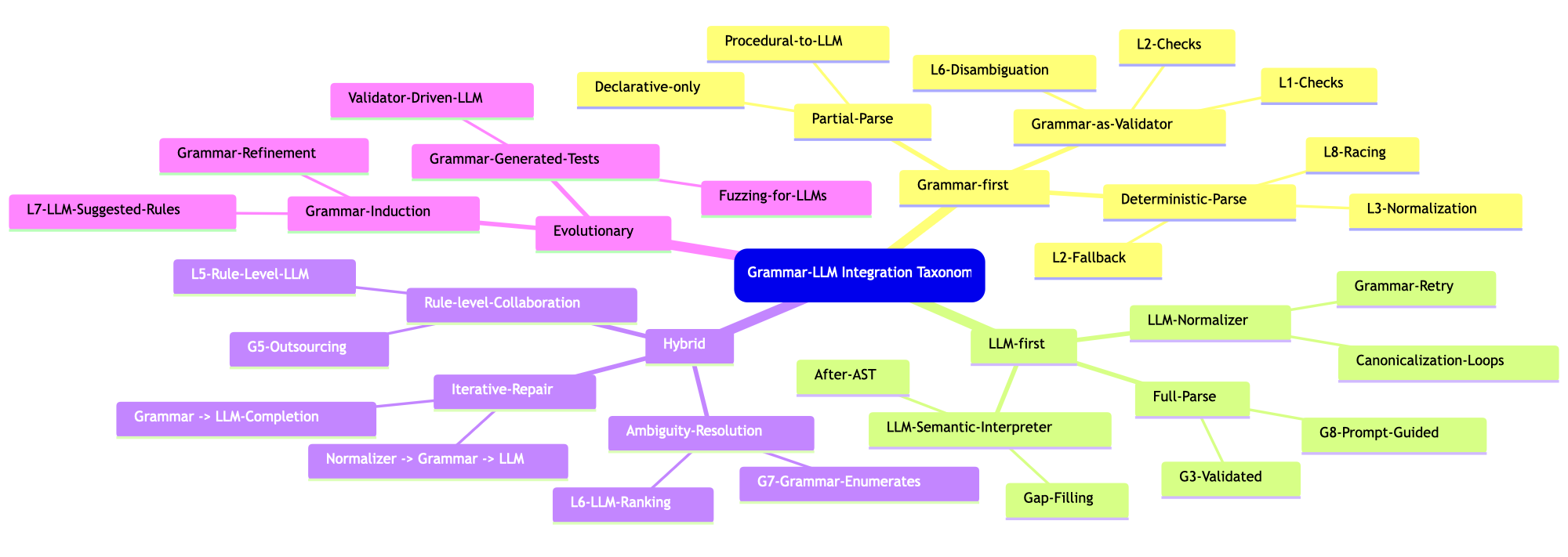
This section has a “concise” table that expands the combinations list above into the main combinatorial strategies for Grammar *** LLMs** for robust parsing and interpretation of workflow specifications. The table is not an exhaustive list of such combinations, but illustrates their diversity and, hopefully, can give ideas for future developments.

A few summary points (for table’s content/subject):

  • Grammar (Raku regex/grammar)
    • Pros: fast, deterministic, validated, reproducible
    • Cons: hard to design for large domains, brittle for natural language inputs
  • LLMs
    • Pros: fast to prototype, excellent at normalization/paraphrasing, flexible
    • Cons: slow, occasionally wrong, hallucination risk, inconsistent output formats
  • Conclusion:
    • The most robust systems combine grammar precision with LLM adaptability , typically by putting grammars first and using LLMs for repair, normalization, expansions, or semantic interpretation (i.e. “fallback”.)

Table: Combination Patterns for Parsing Workflow Specifications

tbl = Dataset[{<|"ID" -> 1, "CombinationPattern" -> "Parallel Race: Grammar + LLM", "Description" -> "Launch grammar-based parsing and one or more LLM interpreters in parallel; whichever yields a valid parse first is accepted.", "Pros" -> {"Fast when grammar succeeds", "Robust fallback", "Reduces latency unpredictability of LLMs"}, "ConsTradeoffs" -> {"Requires orchestration", "Need a validator for LLM output"}|>, <|"ID" -> 2, "CombinationPattern" -> "Grammar-First, LLM-Fallback", "Description" -> "Try grammar parser first; if it fails, invoke LLM-based parsing or normalization.", "Pros" -> {"Deterministic preference for grammar", "Testable correctness when grammar succeeds"}, "ConsTradeoffs" -> {"LLM fallback may produce inconsistent structures"}|>, <|"ID" -> 3, "CombinationPattern" -> "LLM-Assisted Grammar (Rule-Level)", "Description" -> "Individual grammar rules delegate to an LLM for ambiguous or context-heavy matching; LLM supplies tokens or AST fragments.", "Pros" -> {"Handles complexity without inflating grammar", "Modular LLM usage"}, "ConsTradeoffs" -> {"LLM behavior may break rule determinism", "Harder to reproduce"}|>, <|"ID" -> 4, "CombinationPattern" -> "LLM Normalizer -> Grammar Parser", "Description" -> "When grammar fails, LLM rewrites/normalizes input into a canonical form; grammar is applied again.", "Pros" -> {"Grammar remains simple", "Leverages LLM skill at paraphrasing"}, "ConsTradeoffs" -> {"Quality depends on normalizer", "Feedback loops possible"}|>, <|"ID" -> 5, "CombinationPattern" -> "Hybrid Declarative vs Procedural Parsing", "Description" -> "Grammar extracts structural/declarative parts; LLM interprets procedural/stepwise parts or vice versa.", "Pros" -> {"Each subsystem tackles what it's best at", "Reduces grammar complexity"}, "ConsTradeoffs" -> {"Harder to maintain global consistency", "Requires AST stitching logic"}|>, <|"ID" -> 6, "CombinationPattern" -> "Grammar-Generated Tests for LLM", "Description" -> "Grammar used to generate examples and counterexamples; LLM outputs are validated against grammar constraints.", "Pros" -> {"Powerful for verifying LLM outputs", "Reduces hallucinations"}, "ConsTradeoffs" -> {"Grammar must encode constraints richly", "Validation pipeline required"}|>, <|"ID" -> 7, "CombinationPattern" -> "LLM as Adaptive Heuristic for Grammar Ambiguities", "Description" -> "When grammar yields multiple parses, LLM chooses or ranks the \"most plausible\" AST.", "Pros" -> {"Improves disambiguation", "Good for underspecified workflows"}, "ConsTradeoffs" -> {"LLM can pick syntactically impossible interpretations"}|>, <|"ID" -> 8, "CombinationPattern" -> "LLM as Semantic Phase After Grammar", "Description" -> "Grammar creates an AST; LLM interprets semantics, fills in missing steps, or resolves vague ops.", "Pros" -> {"Clean separation of syntax vs semantics", "Grammar ensures correctness"}, "ConsTradeoffs" -> {"Semantic interpretation may drift from syntax"}|>, <|"ID" -> 9, "CombinationPattern" -> "Self-Healing Parse Loop", "Description" -> "Grammar fails -> LLM proposes corrections -> grammar retries -> if still failing, LLM creates full AST.","Pros" -> {"Iterative and robust", "Captures user intent progressively"}, "ConsTradeoffs" -> {"More expensive; risk of oscillation"}|>, <|"ID" -> 10, "CombinationPattern" -> "Grammar Embedding Inside Prompt Templates", "Description" -> "Grammar definitions serialized into the prompt, guiding the LLM to conform to the grammar (soft constraints).", "Pros" -> {"Faster than grammar execution in some cases", "Encourages consistent structure"}, "ConsTradeoffs" -> {"Weak guarantees", "LLM may ignore grammar"}|>, <|"ID" -> 11, "CombinationPattern" -> "LLM-Driven Grammar Induction or Refinement", "Description" -> "LLM suggests new grammar rules or transformations; developer approves; the grammar evolves over time.", "Pros" -> {"Faster grammar evolution", "Useful for new workflow languages"}, "ConsTradeoffs" -> {"Requires human QA", "Risk of regressing accuracy"}|>, <|"ID" -> 12, "CombinationPattern" -> "Regex Engine as LLM Guardrail", "Description" -> "Regex or token rules used to validate or filter LLM results before accepting them.", "Pros" -> {"Lightweight constraints", "Useful for quick prototyping"}, "ConsTradeoffs" -> {"Regex too weak for complex syntax"}|>}]; 
  
 tbl = tbl[All, KeyDrop[#, "ID"] &];
 tbl = tbl[All, ReplacePart[#, "Pros" -> ColumnForm[#Pros]] &];
 tbl = tbl[All, ReplacePart[#, "ConsTradeoffs" -> ColumnForm[#ConsTradeoffs]] &];
 tbl = tbl[All, Style[#, FontFamily -> "Times New Roman"] & /@ # &];
 ResourceFunction["GridTableForm"][tbl]

#CombinationPatternDescriptionProsConsTradeoffs
1Parallel Race: Grammar + LLMLaunch grammar-based parsing and one or more LLM interpreters in parallel; whichever yields a valid parse first is accepted.{{Fast when grammar succeeds}, {Robust fallback}, {Reduces latency unpredictability of LLMs}}{{Requires orchestration}, {Need a validator for LLM output}}
2Grammar-First, LLM-FallbackTry grammar parser first; if it fails, invoke LLM-based parsing or normalization.{{Deterministic preference for grammar}, {Testable correctness when grammar succeeds}}{{LLM fallback may produce inconsistent structures}}
3LLM-Assisted Grammar (Rule-Level)Individual grammar rules delegate to an LLM for ambiguous or context-heavy matching; LLM supplies tokens or AST fragments.{{Handles complexity without inflating grammar}, {Modular LLM usage}}{{LLM behavior may break rule determinism}, {Harder to reproduce}}
4LLM Normalizer -> Grammar ParserWhen grammar fails, LLM rewrites/normalizes input into a canonical form; grammar is applied again.{{Grammar remains simple}, {Leverages LLM skill at paraphrasing}}{{Quality depends on normalizer}, {Feedback loops possible}}
5Hybrid Declarative vs Procedural ParsingGrammar extracts structural/declarative parts; LLM interprets procedural/stepwise parts or vice versa.{{Each subsystem tackles what it’s best at}, {Reduces grammar complexity}}{{Harder to maintain global consistency}, {Requires AST stitching logic}}
6Grammar-Generated Tests for LLMGrammar used to generate examples and counterexamples; LLM outputs are validated against grammar constraints.{{Powerful for verifying LLM outputs}, {Reduces hallucinations}}{{Grammar must encode constraints richly}, {Validation pipeline required}}
7LLM as Adaptive Heuristic for Grammar AmbiguitiesWhen grammar yields multiple parses, LLM chooses or ranks the “most plausible” AST.{{Improves disambiguation}, {Good for underspecified workflows}}{{LLM can pick syntactically impossible interpretations}}
8LLM as Semantic Phase After GrammarGrammar creates an AST; LLM interprets semantics, fills in missing steps, or resolves vague ops.{{Clean separation of syntax vs semantics}, {Grammar ensures correctness}}{{Semantic interpretation may drift from syntax}}
9Self-Healing Parse LoopGrammar fails -> LLM proposes corrections -> grammar retries -> if still failing, LLM creates full AST.{{Iterative and robust}, {Captures user intent progressively}}{{More expensive; risk of oscillation}}
10Grammar Embedding Inside Prompt TemplatesGrammar definitions serialized into the prompt, guiding the LLM to conform to the grammar (soft constraints).{{Faster than grammar execution in some cases}, {Encourages consistent structure}}{{Weak guarantees}, {LLM may ignore grammar}}
11LLM-Driven Grammar Induction or RefinementLLM suggests new grammar rules or transformations; developer approves; the grammar evolves over time.{{Faster grammar evolution}, {Useful for new workflow languages}}{{Requires human QA}, {Risk of regressing accuracy}}
12Regex Engine as LLM GuardrailRegex or token rules used to validate or filter LLM results before accepting them.{{Lightweight constraints}, {Useful for quick prototyping}}{{Regex too weak for complex syntax}}

Diversity reasons

  • The diversity of combinations in the table above arises because Raku grammars and LLMs occupy fundamentally different but highly complementary positions in the parsing spectrum.
  • Raku grammars provide determinism, speed, verifiability, and structural guarantees, but they require upfront design and struggle with ambiguity, informal input, and evolving specifications.
  • LLMs, in contrast, excel at normalization, semantic interpretation, ambiguity resolution, and adapting to fluid or poorly defined languages, yet they lack determinism, may hallucinate, and are slower.
  • When these two technologies meet, every architectural choice — who handles syntax, who handles semantics, who runs first, who validates whom, who repairs or refines — defines a distinct strategy.
  • Hence, the design space naturally expands into many valid hybrid patterns rather than a single “best” pipeline.
  • That said, the fallback pattern implemented below can be considered the “best option” from certain development perspectives because it is simple, effective, and has fast execution times.

See the corresponding Morphological Analysis table which correspond to this taxonomy mind-map:

Setup

Here are the packages used in this document (notebook):

Needs["AntonAntonov`DSLTranslation`"];
Needs["AntonAntonov`NLPTemplateEngine`"];
Needs["AntonAntonov`DSLExamples`"];
Needs["AntonAntonov`MermaidJS`"];
Needs["AntonAntonov`MonadicSparseMatrixRecommender`"];

Three DSL translations

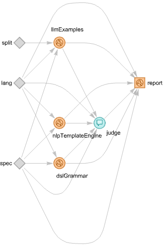
This section demonstrates the use of three different translation methods:

  1. Grammar-based parser-interpreter of computational workflows
  2. LLM-based translator using few-shot learning with relevant DSL examples
  3. Natural Language Processing (NLP) interpreter using code templates and LLMs to fill-in the corresponding parameters

The translators are ordered according of their faithfulness, most faithful first. It can be said that at the same time, the translators are ordered according to their coverage — widest coverage is by the last.

Grammar-based

Here a recommender pipeline specified with natural language commands is translated into Raku code of the package “ML::SparseMatrixRecommender” using a sub of the paclet “DSLTranslation”:

spec = "create from dsData; apply LSI functions IDF, None, Cosine; recommend by profile for passengerSex:male, and passengerClass:1st; join across using dsData; echo the pipeline value";

DSLTranslation[spec, "WLCode" -> True]

Out[]= SMRMonUnit[]==>SMRMonCreate[dsData]==>SMRMonApplyTermWeightFunctions["GlobalWeightFunction" -> "IDF", "LocalWeightFunction" -> "None", "NormalizerFunction" -> "Cosine"]==>SMRMonRecommendByProfile[{"passengerSex:male", "passengerClass:1st"}]==>SMRMonJoinAcross[dsData]==>SMRMonEchoValue[]

The function DSLTranslation uses a web service by default but if Raku and the package “DSL::Translators” are installed it can use the provided Command Line Interface (CLI):

DSLTranslation[spec, "Source" -> "Shell", "CLIPath" -> "~/.rakubrew/shims/dsl-translation"]

Out[]= SMRMonUnit[]==>SMRMonCreate[dsData]==>SMRMonApplyTermWeightFunctions["GlobalWeightFunction" -> "IDF", "LocalWeightFunction" -> "None", "NormalizerFunction" -> "Cosine"]==>SMRMonRecommendByProfile[{"passengerSex:male", "passengerClass:1st"}]==>SMRMonJoinAcross[dsData]==>SMRMonEchoValue[]

For more details of the grammar-based approach see the presentations:

Via LLM examples

LLM translations can be done using a set of from-to rules. This is the so-called few shot learning of LLMs. The paclet “DSLExamples” has a collection of such examples for different computational workflows. (Mostly ML at this point.) The examples are hierarchically organized by programming language and workflow name; see the resource file “dsl-examples.json”, or execute DSLExamples[].

Here is a table that shows the known DSL translation examples in “DSL::Examples” :

Dataset[Map[Flatten, List @@@ Normal[ResourceFunction["AssociationKeyFlatten"][Map[Length, DSLExamples[], {2}]]]]][All, AssociationThread[{"Language", "Workflow", "Count"}, #] &]

LanguageWorkflowCount
WLClCon20
WLQRMon27
WLLSAMon17
WLSMRMon20
PythonQRMon23
PythonLSAMon15
PythonSMRMon20
RQRMon26
RLSAMon17
RSMRMon20
RakuSMRMon20

Here is the definition of an LLM translation function that uses examples:

LLMPipelineSegment[lang_String : "WL", workflow_String : "SMRMon"] := LLMExampleFunction[Normal@DSLExamples[lang, workflow]];

Here is a recommender pipeline specified with natural language commands:

spec = "new recommender; create from @dsData;  apply LSI functions IDF, None, Cosine;  recommend by profile for passengerSex:male, and passengerClass:1st; join across with @dsData on \"id\"; echo the pipeline value; classify by profile passengerSex:female, and passengerClass:1st on the tag passengerSurvival; echo value";

commands = StringSplit[spec, ""];

Translate to WL code line-by-line:

res = LLMPipelineSegment[] /@ commands; res = Map[StringTrim@StringReplace[#, RegularExpression["Output\h*:"] -> ""] &, res];
 res = StringRiffle[res, "==>"]

Out[]= "SMRMonUnit[]==>SMRMonCreate[dsData]==>SMRMonApplyTermWeightFunctions[\"IDF\", \"None\", \"Cosine\"]==>SMRMonRecommendByProfile[{\"passengerSex.male\", \"passengerClass.1st\"}]==>SMRMonJoinAcross[@dsData, \"id\"]==>SMRMonEchoValue[]==>SMRMonClassify[\"passengerSurvival\", {\"passengerSex.female\", \"passengerClass.1st\"}]==>SMRMonEchoValue[]"

Or translate by just calling the function over the whole $spec :

LLMPipelineSegment[][spec]

Out[]= "```wolframSMRMonUnit[] |> SMRMonCreate[dsData] |> SMRMonApplyTermWeightFunctions[\"IDF\", \"None\", \"Cosine\"] |> SMRMonRecommendByProfile[{\"passengerSex\" -> \"male\", \"passengerClass\" -> \"1st\"}] |> SMRMonJoinAcross[dsData, \"id\"] |> SMRMonEchoValue[] |> SMRMonClassify[\"passengerSurvival\", {\"passengerSex\" -> \"female\", \"passengerClass\" -> \"1st\"}] |> SMRMonEchoValue[]```"

Remark: That latter call is faster, but it needs additional processing for “monadic” workflows.

By NLP Template Engine

Here a “free text” recommender pipeline specification is translated to Raku code using the sub concretize of the package “ML::NLPTemplateEngine” :

Concretize["create a recommender with dfTitanic; apply the LSI functions IDF, None, Cosine; recommend by profile 1st and male"]

Out[]= Hold[smrObj = SMRMonUnit[]==>SMRMonCreate[None]==>SMRMonRecommendByProfile[{"1st", "male"}, profile]==>SMRMonJoinAcross[None]==>SMRMonEchoValue[];]

The paclet “NLPTemplateEngine” uses a Question Answering System (QAS) implemented in FindTextualAnswer. A QAS can be implemented in different ways, with different conceptual and computation complexity. “NLPTemplateEngine” also has an LLM based implementation of QAS, LLMTextualAnswer. (Also see the resource function with the same name.)

For more details of the NLP template engine approach see the presentations:

Parallel race (judged): Grammar + LLM

In this section we implement the first, most obvious, and conceptually simplest combination of grammar-based- with LLM-based translations:

  • All translators — grammar-based and LLM-based are run in parallel
  • An LLM judge selects the one that adheres best to the given specification

The implementation of this strategy with an LLM graph (say, by using LLMGraph) is straightforward.

Here is such an LLM graph that:

  • Runs all three translation methods above
  • There is a judge that picks which on of the LLM methods produced better result
  • Judge’s output is used to make (and launch) a notebook report
LLMPipelineSegmentFunction[lang_ : "WL", worflowName_String : "SMRMon"] := LLMExampleFunction[Normal@DSLExamples[][lang][worflowName]];

aLangSeparator = <| "Python" -> ".", "Raku" -> ".", "R" -> "%>%", "WL" -> "==>" |>;

Clear[LLMExamplesTranslation];
 LLMExamplesTranslation[spec_, lang_ : "WL", worflowName_String : "SMRMon", splitQ_ : False] := 
    Module[{llmPipelineSegment, commands}, 
     
     llmPipelineSegment = LLMPipelineSegmentFunction[lang]; 
     
     If[TrueQ@splitQ, 
      Echo["with spec splitting..."]; 
      commands = StringSplit[spec, ""]; 
      StringRiffle[StringTrim@StringReplace[llmPipelineSegment /@ commands, StartOfString ~~ "Output" ~~ ___ ~~ ":" -> ""], aLangSeparator[lang]], 
     (*ELSE*) 
      Echo["no spec splitting..."]; 
      StringReplace[llmPipelineSegment[spec], ";" -> aLangSeparator[lang], Infinity] 
     ] 
    ];

JudgeFunction[spec_, lang_, dslGrammar_, llmExamples_, nlpTemplateEngine_] := 
    StringRiffle[{
      "Choose the generated code that most fully adheres to the spec:", 
      spec, 
      "from the following " <> lang <> " generation results:", "1) DSL-grammar:" <> dslGrammar <> "", 
      "2) LLM-examples:" <> llmExamples <> "", 
      "3) NLP-template-engine:" <> nlpTemplateEngine <> "", 
      "and copy it:" 
     }, 
     "" 
    ];

(*JudgeFunction[`spec`,`lang`,`dslGrammar`,`llmExamples`,`nlpTemplateEngine`]*)

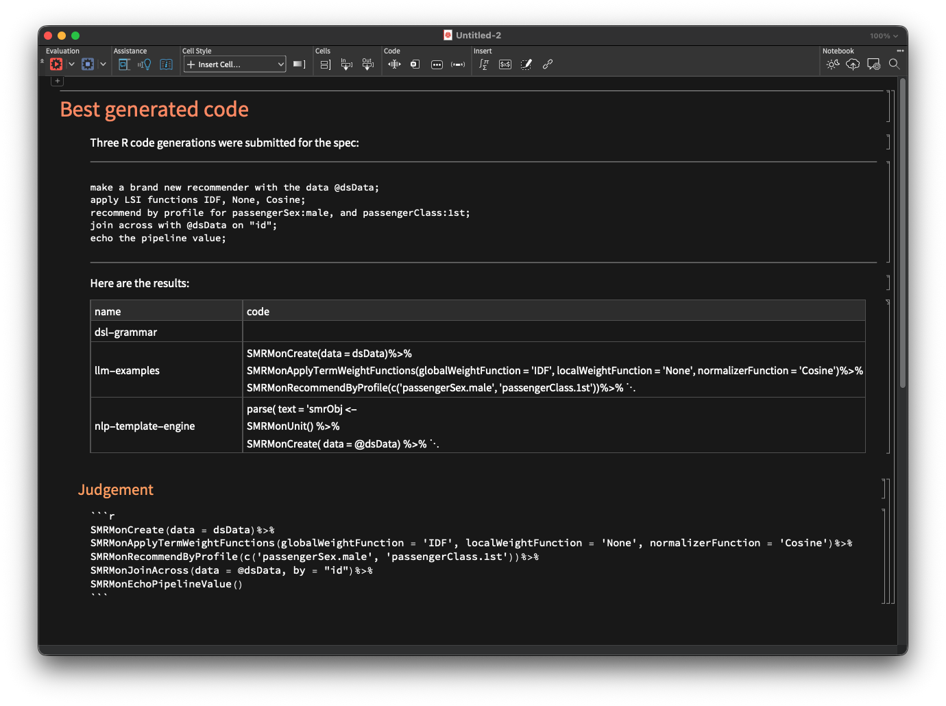
tmplJudge = StringTemplate["Choose the generated code that most fully adheres to the spec:\\n\\n\\n`spec`\\n\\n\\nfrom the following `lang` generation results:\\n\\n\\n1) DSL-grammar:\\n`dslGrammar`\\n\\n\\n2) LLM-examples:\\n`llmExamples`\\n\\n\\n3) NLP-template-engine:\\n`nlpTemplateEngine`\\n\\n\\nand copy it:"]

1sk1d044my02q
JudgementReport[spec_, lang_, dslGrammar_, llmExamples_, nlpTemplateEngine_, judge_] := 
    Module[{names, codes, rows, tableHTML, judgementBlock}, 
     names = {"dsl-grammar", "llm-examples", "nlp-template-engine"}; 
     codes = {dslGrammar, llmExamples, nlpTemplateEngine}; 
     rows = MapThread[<|"name" -> #1, "code" -> #2|> &, {names, codes}];
    (*WL analogue of to-html(...,field-names=> <name code>)*) 
     tableHTML = Dataset[rows]; 
     judgementBlock = If[StringContainsQ[judge, "```"], judge, "```" <> lang <> "" <> judge <> "```"]; 
     CreateDocument[{
       TextCell["Best generated code", "Section"], 
       TextCell["Three " <> lang <> " code generations were submitted for the spec:", "Text"], 
       TextCell[spec, "Program"], 
       TextCell["Here are the results:", "Text"], 
       ExpressionCell[tableHTML, "Output"], 
       TextCell["Judgement", "Subsection"], 
       TextCell[judgementBlock, "Output"] 
      }] 
    ];

Rules for parallel race:

rules = <|
     "dslGrammar" -> <|"EvaluationFunction" -> (DSLTranslation[#spec, "ToLanguage" -> #lang, "WLCode" -> False, "Format" -> "CODE"] &), "Input" -> {"spec", "lang"}|>, 
     "llmExamples" -> <|"EvaluationFunction" -> (LLMExamplesTranslation[#spec, #lang, "SMRMon", #split] &), "Input" -> {"spec", "lang", "split"}|>,
     "nlpTemplateEngine" -> <|"EvaluationFunction" -> (Concretize[#spec, "TargetLanguage" -> #lang] &), "Input" -> {"spec", "lang"}|>,
    (*judge-><|EvaluationFunction->(judgeFunction[#spec,#lang,#dslGrammar,#llmExamples,#nlpTemplateEngine]&)|>,*) 
     "judge" -> tmplJudge, 
     "report" -> <|"EvaluationFunction" -> (JudgementReport[#spec, #lang, #dslGrammar, #llmExamples, #nlpTemplateEngine, #judge] &)|> 
    |>;

Corresponding LLM-graph construction:

gBestCode = LLMGraph[rules]

1l626dkgaymsq

Here is a recommender workflow specification:

spec = " make a brand new recommender with the data @dsData; apply LSI functions IDF, None, Cosine;  recommend by profile for passengerSex:male, and passengerClass:1st; join across with @dsData on \"id\"; echo the pipeline value; ";

Here the graph is executed:

res = gBestCode[<|"spec" -> spec, "lang" -> "R", "split" -> True|>];

Here is a screenshot of the LLM-graph result:

LLM-graph visualization

Information[gBestCode, "Graph"]

For details on LLM-graphs design see the video:

Fallback: DSL-grammar to LLM-examples

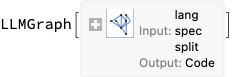
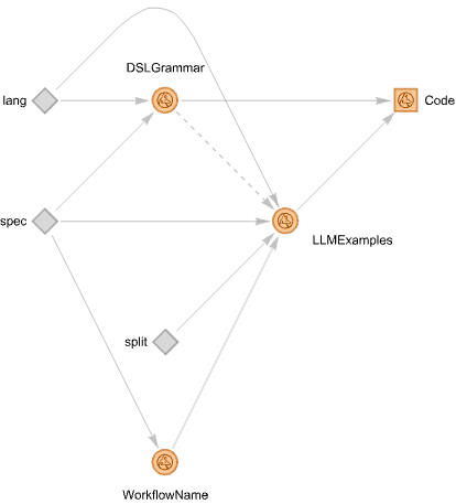
Instead of having DSL-grammar- and LLM computations running in parallel, we can make an LLM-graph in which the LLM computations are invoked if the DSL-grammar parsing-and-interpretation fails. In this section we make such a graph.

Before making the graph let us also generalize it to work with other ML workflows, not just recommendations.

Let us make an LLM function with a similar functionality. I.e. an LLM-function that classifies a natural language computation specification into workflow labels used by “DSLExamples”. Here is such a function using the sub LLMClassify provided by “NLPTemplateEngine”:

lsMLLabels = {"Classification", "Latent Semantic Analysis", "Quantile Regression", "Recommendations"}; 
  
 aWorlflowMonNames = <|
       "Classification" -> "ClCon", 
       "Latent Semantic Analysis" -> "LSAMon", 
       "Quantile Regression" -> "QRMon", 
       "Recommendations" -> "SMRMon" 
     |>; 
  
 LLMWorkflowClassify[spec_] := Module[{res = LLMClassify[spec, lsMLLabels, "Request" -> "which of these workflows characterizes it (just one label)"]}, 
     Lookup[aWorlflowMonNames, res, res] 
   ]

(* Example invocation *)
 (*LLMWorkflowClassify[spec]*)

Remark: The paclet “NLPTemplateEngine” has (1) a pre-trained ML workflows classifier, and (2) a separate, generic LLM-based classifier.

Rules for fallback execution:

TranslationSuccessQ[s_] := StringQ[s] && StringLength[StringTrim[s]] > 5;
 rules = <|
     "DSLGrammar" -> <|"EvaluationFunction" -> (DSLTranslation[#spec, "ToLanguage" -> #lang, "WLCode" -> False, "Format" -> "CODE"] &), "Input" -> {"spec", "lang"}|>, 
     "WorkflowName" -> <|"EvaluationFunction" -> (LLMWorkflowClassify[#spec] &)|>, 
     "LLMExamples" -> <|
       "EvaluationFunction" -> (LLMExamplesTranslation[#spec, #lang, #WorkflowName, #split] &), 
       "Input" -> {"spec", "lang", "WorkflowName", "split"}, 
       "TestFunction" -> (! TranslationSuccessQ[#DSLGrammar] &)|>, 
     "Code" -> <|"EvaluationFunction" -> (If[TranslationSuccessQ[#DSLGrammar], #DSLGrammar, #LLMExamples] &)|> 
    |>;

Corresponding LLM-graph construction:

gRobust = LLMGraph[rules]

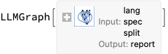
Here the LLM graph is run over a spec that can be parsed by DSL-grammar (notice the very short computation time):

Here is the obtained result:

Here is a spec that cannot be parsed by the DSL-grammar interpreter — note that there is just a small language change in the first line:

spec = " create from @dsData;  apply LSI functions IDF, None, Cosine;  recommend by profile for passengerSex:male, and passengerClass:1st; join across with @dsData on \"id\"; echo the pipeline value; ";

Nevertheless, we obtain a correct result via LLM-examples:

res = gRobust[<|"spec" -> spec, "lang" -> "R", "split" -> True|>]

Out[]= "SMRMonCreate(data = @dsData) %>%SMRMonApplyTermWeightFunctions(globalWeightFunction = \"IDF\", localWeightFunction = \"None\", normalizerFunction = \"Cosine\") %>%SMRMonRecommendByProfile( profile = c(\"passengerSex:male\", \"passengerClass:1st\")) %>%SMRMonJoinAcross( data = @dsData, by = \"id\" ) %>%SMRMonEchoValue()"

Here is the corresponding graph plot:

Information[gRobust, "Graph"]

Let us specify another workflow — for ML-classification with Wolfram Language — and run the graph:

spec = " use the dataset @dsData; split the data into training and testing parts with 0.8 ratio; make a nearest neighbors classifier; show classifier accuracy, precision, and recall; echo the pipeline value; ";

res = gRobust[<|"spec" -> spec, "lang" -> "WL", "split" -> True|>]

Out[]= "SMRMonUse[dsData]==>SMRMonSplitData[0.8]==>SMRMonMakeClassifier[\"NearestNeighbors\"]==>SMRMonClassifierMeasurements[\"Accuracy\", \"Precision\", \"Recall\"]==>SMRMonEchoValue[]"

Concluding comments and observations

  • Using LLM graphs gives the ability to impose desired orchestration and collaboration between deterministic programs and LLMs.
    • By contrast, the “inversion of control” of LLM – tools is “capricious.”
  • LLM-graphs are both a generalization of LLM-tools, and a lower level infrastructural functionality than LLM-tools.
  • The LLM-graph for the parallel-race translation is very similar to the LLM-graph for comprehensive document summarization described in [AA4].
  • The expectation that DSL examples would provide both fast and faithful results is mostly confirmed in ≈20 experiments.
  • Using the NLP template engine is also fast because LLMs are harnessed through QAS.
  • The DSL examples translation had to be completed with a workflow classifier.
    • Such classifiers are also part of the implementations of the other two approaches .
    • The grammar – based one uses a deterministic classifier, [AA1]
    • The NLP template engine uses an LLM classifier .
  • An interesting extension of the current work is to have a grammar-LLM combination in which when the grammar fails then the LLM “normalizes” the specs until the grammar can parse them.
    • Currently, LLMGraph does not support graphs with cycles, hence this approach “can wait” (or be implemented by other means .)
  • Multiple DSL examples can be efficiently derived by random sentence generation with different grammars.
    • Similar to the DSL commands classifier making approach taken in [AA1] .
  • LLMs can be also used to improve and extend the DSL grammars.
    • And it is interesting to consider automating that process, instead of doing it via human supervision.
  • This notebook is the Wolfram Language version of the document “Day 6 — Robust code generation combining grammars and LLMs”, [AA6], (notebook), using Raku.

References

Articles, blog posts

[AA1] Anton Antonov, “Fast and compact classifier of DSL commands” , (2022), RakuForPrediction at WordPress .

[AA2] Anton Antonov, “Grammar based random sentences generation, Part 1” , (2023), RakuForPrediction at WordPress .

[AA3] Anton Antonov, “LLM::Graph” , (2025), RakuForPrediction at WordPress .

[AA4] Anton Antonov, “Agentic-AI for text summarization” , (2025), RakuForPrediction at WordPress .

[AA5] Anton Antonov, “LLM::Graph plots interpretation guide” , (2025), RakuForPrediction at WordPress .

[AA6] Anton Antonov, “Day 6 — Robust code generation combining grammars and LLMs”, (2025), Raku Advent Calendar at WordPress.

Packages

[AAp1] Anton Antonov, DSL::Translators, Raku package , (2020-2025), GitHub/antononcube .

[AAp2] Anton Antonov, ML::FindTextualAnswer, Raku package , (2023-2025), GitHub/antononcube .

[AAp3] Anton Antonov, MLP::NLPTemplateEngine, Raku package , (2023-2025), GitHub/antononcube .

[AAp4] Anton Antonov, DSL::Examples, Raku package , (2024-2025), GitHub/antononcube .

[AAp5] Anton Antonov, LLM::Graph, Raku package , (2025), GitHub/antononcube .

[AAp6] Anton Antonov, ML::SparseMatrixRecommender, Raku package , (2025), GitHub/antononcube .

Videos

[AAv1] Anton Antonov, “Raku for Prediction presentation at The Raku Conference 2021”, (2021), YouTube/@AAA4prediction .

[AAv2] Anton Antonov, “Simplified Machine Learning Workflows Overview”, (2022), YouTube/@WolframResearch .

[AAv3] Anton Antonov, “NLP Template Engine, Part 1” , (2021), YouTube/@AAA4prediction .

[AAv4] Anton Antonov, “Natural Language Processing Template Engine” , (2023), YouTube/@WolframResearch .

[WRIv1] Wolfram Research, Inc., “Live CEOing Ep 886: Design Review of LLMGraph” , (2025), YouTube/@WolframResearch .