Simple time series conversational engine

Introduction

In this blog post I am going to discuss the creation (design and programming) of a simple conversational engine for time series analysis. The conversational engine responds to commands for:
1. loading time series data (weather data, stock data, or data files),
2. finding outliers,
3. analysis by curve fitting,
4. plotting, and
5. help and state changes.

This blog post is related to the blog post [1] and uses the package with functional parsers [2] and the Quantile regression package [3].

I programmed this engine ten months ago and here is link to a movie that demonstrates it, [4]: https://www.youtube.com/watch?v=wlZ5ANglVI4 .

A package with all of the code of the conversational engine can be downloaded from GitHub, [12] and executed with Import:


Import["https://raw.githubusercontent.com/antononcube/MathematicaForPrediction/master/Examples/SimpleTimeSeriesConversationalEngine.m"]


More about functional parsers, which were essential for the building of the conversational engine, can be read in “Functional parsers” by Fokker, [5].

Design of the conversational engine

The conversational engine is a finite state machine. It has a command recognizer state and command application state. The switching between the states is done upon completion states functions. The recognized commands are English sentences. Some of the sentences include Mathematica code.

Let use describe the structure of the conversational engine.

States

1. Acceptor state
The Acceptor state parses and recognizes commands. If the given command is successfully parsed then the parsing result is given to the Transducer state. Otherwise a message “Unknown command” is emitted and no state change is made (i.e.we are still in the Acceptor state).

2. Transducer state
Interprets the parsed a command by the Acceptor state. This state emits different messages according to the loaded data and accumulated graphics objects.

The states are named according to the classification given in the Wikipedia article about finite-state machines, [5]. According to that classification the conversational engine is a Mealy machine.

Responses

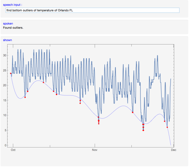
The results of the applied time series analysis are graphical. The Transducer state accumulates the graphs of the commands and displays them with the data. The conversational engine responses have a spoken part and a graphics part. The responses have at least a spoken part. The graphics part can omitted.

Commands

The weather data commands can be for temperature, wind speed, and pressure over a specified city. For example, “load temperature of Atlanta” or “load the Chicago wind speeds”.

The financial data commands can be for stock price or trading volume. For example, “load trade volume of NYSE:GOOG” or “load stock price of NYSE:APPL”.

The weather and stocks data loading commands do not take time period, they take only city and company specifications for WeatherData and FinancialData respectively.

The loading of data files is done with commands like “load file ‘~/LogDataWithSkewedNoise.csv’ “.

The time series analysis commands we consider are: curve fitting by a list specified functions, finding regression quantiles, and finding outliers. For example, “compute least squares fit of {1,x,Sin[x/10^6]}”, “compute 5 regression quantiles”, “find top outliers”.

The graphics commands are “plot data”, “plot(s) joined”, “plot(s) not joined”, “clear graphics”.

In addition, the conversational engine takes global, service commands like “help”, “all commands”, “start over’, etc.

Grammar specification

In order to respond to the commands that are English sentences we have to be able to parse these sentences into concrete state or message specifications. This means that we have to define the grammatical structures of the command sentences and the words in them.

This section describes the grammar of the commands using Extended Backus-Naur Form (EBNF). The package FunctionalParsers.m, [2], has Mathematica functions that generate parsers from EBNF of a grammar (see [9] and the next section). The resulting parsers are used in the conversational engine described above.

Commands for loading data explanations

Let us explain the derivation and rationale of the grammar rules for the data loading commands. (I am not going to describe all the language considerations and decisions I have made for the commands grammar. These decisions can be traced in the EBNF grammar specification.)

We want to parse and interpret commands like:
1. load data file ‘timeTable.csv’ ,
2. load temperature of Atlanta ,
3. load the wind speeds of Chicago ,
4. load the stock price of NYSE:APPL ,
5. load trading volume of NYSE:GOOG .

We can see that we have three different types of data loading commands: for files, for weather data, and for financial data. Each of these commands when parsed would be easy to interpret using Mathematica’s functions Import, WeatherData, and FinancialData respectively. Note that — because we want to keep the grammar simple — for the weather and financial data there is no time period specification. For the weather data we are going to load data for the last 60 days; for the financial data for the last 365 days. Also, for simplicity, we are not going to consider data loading commands that start with the phrases “get”, “get me”, “please load”, etc.

To this end the general load data command structure is:

Note that in the grammar rules above some of the words are optional; the optional words are put within square brackets. With the first rule we have separated the file loading from the weather and financial data loading. The file loading is further specified with rule 2. Rule 3 separates the preamble of the weather and financial data loading commands from the data specification. The latter is partitioned in rule 4. Rule 5 gives all of the possible data type requests for the weather data: temperature, pressure, and wind speed. Rule 6 gives the two possible types for financial data requests: stock price and trade volume. The file name, city, and company specifications are left out, but the rules for them are be easy to formulate.

The command grammar used in the conversational engine uses additional data loading definitions and allows “reverse” data load commands like: “load the Chicago wind speeds”.

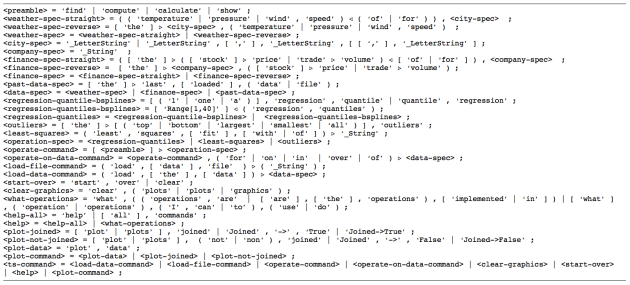
Full grammar specification

In this sub-section the full grammar specification is given. Note that some parts of the commands are specified to be dropped from the parsing results using the symbols “\[RightTriangle]” and “\[LeftTriangle]”. (For example ” ‘trade’ \[RightTriangle] ‘volume’ ” means “parse the sequence of words ‘trade’ ‘volume’ and return ‘volume’ as a result”.) The specification ‘_LetterString’ is an implementation shortcut for matching words and identifiers with the package FunctionalParsers.m, [2].

The rules were simplified for clarity, the actual conversational engine code can be retrieved, [8].

The grammar specified above takes complicated commands like “find regression quantiles over temperature of Atlanta”.

(In certain cases I prefer reading grammars in EBNF using Emacs and ebnf-mode.el, [7].)

Parsers for the grammar

Using the grammar specification [8] and the package FunctionalParsers.m, [2], we can generate the parsers for that grammar. A detailed description of the parser generation process is given in [9].

Here is the generation step:


tokens = ToTokens[timeSeriesEBNFCode];
res = GenerateParsersFromEBNF[tokens];
res // LeafCount

Out[4]= 3069


The generation step creates a set of parsers:

In[16]:= Magnify[Shallow[res[[1, 1, 2]], 6], 0.8]

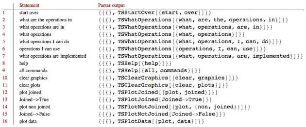
Here are the parsing results returned by the “master” rule pTSCOMMAND:

Here is another list for the engine’s “service” commands:

And see their parsing outcome using the function ParsingTestTable provided by FunctionalParsers.m:

questions = {"load data file '~/example.csv'",
"load file '~/anotherExample.csv'"};
ParsingTestTable[ParseShortest[pLOADFILECOMMAND], questions]

Note that the parser takes commands with Mathematica expressions parts if those expressions are written without spaces:

questions = {"least squares fit with x+Sin[x]"};
ParsingTestTable[ParseShortest[pTSCOMMAND], questions]

This type of commands are specified with the grammar rule:

= ( ‘least’ , ‘squares’ , [ ‘fit’ ] , [ ‘with’ | ‘of’ ] ) \[RightTriangle] ‘_String’ ;

Interpreters (for the parsers)

Next we have to write interpreters for the parsing results. Note that the parsing results are Mathematica expressions with heads that hint to the semantic meaning behind the parsed commands. Since we are viewing the conversational engine as a finite state machine we can say that for each parsing result we have to write a function that “reacts” to result’s head and content. This is a fairly straightforward process very similar to the one described by the Interpreter design pattern, [10].

A package with all of the code of the conversational engine can be downloaded from GitHub, [12]. The interpreters code can be found in the section “Interpreters”.

The conversational engine programming

The conversational engine was programmed using Mathematica’s dynamic evaluation functions and mechanisms. The implementation follows the Absorber and Transductor state design described above in the section “Design of the conversational engine”.

The engine has three panels: for command input, for spoken output, and for graphical output. It is fully demonstrated with the movie “Time series conversational engine” posted on YouTube, [4].

As it was mentioned in the introduction the engine can be run using Import:

Import[“https://raw.githubusercontent.com/antononcube/MathematicaForPrediction/master/Examples/SimpleTimeSeriesConversationalEngine.m”%5D

Future plans

The engine can be extended in many directions depending on the final goals for it.

One must have extension is the ability to take time period specifications for the weather and financial data.

The time series analysis can be extended with more detailed analysis using functions like TimeSeriesModelFit or heteroscedasticity analysis using multiple regression quantiles, [11].

A third set of extensions is the ability to load additional kinds of data, like, the evolutions of countries populations or gross domestic products.

References

[1] Anton Antonov, Natural language processing with functional parsers, blog post at WordPress, (2014).

[2] Anton Antonov, Functional parsers Mathematica package, source code at GitHub, https://github.com/antononcube/MathematicaForPrediction, package FunctionalParsers.m, (2014).

[3] Anton Antonov, Quantile regression Mathematica package, source code at GitHub, https://github.com/antononcube/MathematicaForPrediction, package QuantileRegression.m, (2013).

[4] Anton Antonov, Time series conversational engine, a YouTube movie.

[5] Wikipedia entry: Finite-state Machine, http://en.wikipedia.org/wiki/Finite-state_machine .

[6] Jeroen Fokker, Functional parsers, In: Advanced Functional Programming, Tutorial text of the First international spring school on advanced functional programming techniques in Båstad, Sweden, may 1995. (Johan Jeuring and Erik Meijer, eds). Berlin, Springer 1995 (LNCS 925), pp. 1-23. http://www.staff.science.uu.nl/~fokke101/article/parsers/index.html .

[7] Jeramey Crawford, Extended Backus-Naur Form Mode, ebnf-mode.el, emacs LISP at Github, https://github.com/jeramey/ebnf-mode .

[8] Anton Antonov, Time series conversational engine grammar in EBNF, TimeSeriesConversationalEngineGrammar.ebnf at the MathematicaForPrediction project at GitHub.

[9] Anton Antonov, Functional parsers for an integration requests language, PDF document at GitHub, https://github.com/antononcube/MathematicaForPrediction/tree/master/Documentation , (2014).

[10] Erich GammaTaligent, Richard Helm, Ralph Johnson, John Vlissides, Design patterns: elements of reusable object-oriented softwareAddison-Wesley Longman Publishing Co., Inc. Boston, MA, USA ©1995, ISBN:0-201-63361-2, http://en.wikipedia.org/wiki/Design_Patterns .

[11] Anton Antonov, Estimation of conditional density distributions, “Mathematica for prediction algorithms” blog at WordPress, (2014).

[12] Anton Antonov, Simple Time Series Conversational Engine Mathematica package, SimpleTimeSeriesConversationalEngine.m at the MathematicaForPrediction project at GitHub.