Introduction
The main goal of this notebook is to provide some basic views and insights into the landscape of cryptocurrencies. The “landscape” we consider consists of price action and trading volume time series for cryptocurrencies found in Yahoo Finance.
Here is the work plan followed in this notebook:
- Get cryptocurrency data
- Do basic data analysis over suitable date ranges
- Gather important cryptocurrency events
- Plot together cryptocurrency prices and trading volume time series together with the events
- Make observations and conjectures over the plots
- Find “global” correlations between the different cryptocurrencies
- Find clusters of cryptocurrencies based on time series correlations
Here are some details for the steps above:
- The procedure of obtaining the cryptocurrencies data, point 1, is explained in detail in [AA1].
- There is a dedicated resource object CrypocurrencyData that provides cryptocurrency data and related documentation.
- The cryptocurrency events data, point 3, is taken from different news sites.
- Links are provided in the corresponding dataset.
- The points 6 and 7 follow similar explorations (and code) described in [AA2, AA3].
- Those two articles deal with COVID-19 time series.
Remark: Note that in this notebook we do not discuss philosophical, macro-economic, and environmental issues with cryptocurrencies. We only discuss financial time series data.
Cryptocurrencies data
The cryptocurrencies data used in this notebook is obtained from found in Yahoo Finance . The procedure of obtaining the cryptocurrencies data is explained in detail in [AA1]. There is a dedicated resource object CrypocurrencyData that provides the cryptocurrency data and related documentation.
Here are all cryptocurrencies we have data for:
ResourceFunction["CryptocurrencyData"]["CryptocurrencyNames"]

(*<|"BTC" -> "Bitcoin", "ETH" -> "Ethereum", "USDT" -> "Tether", "BNB" -> "BinanceCoin", "ADA" -> "Cardano", "XRP" -> "XRP", "USDC" -> "Coin", "DOGE" -> "Dogecoin", "DOT1" -> "Polkadot", "HEX" -> "HEX", "UNI3" -> "Uniswap", "BCH" -> "BitcoinCash", "LTC" -> "Litecoin", "LINK" -> "Chainlink", "SOL1" -> "Solana", "MATIC" -> "MaticNetwork", "THETA" -> "THETA", "XLM" -> "Stellar", "VET" -> "VeChain", "ICP1" -> "InternetComputer", "ETC" -> "EthereumClassic", "TRX" -> "TRON", "FIL" -> "FilecoinFutures", "XMR" -> "Monero", "EOS" -> "EOS"|>*)
Remark: FinancialData is “aware” of 10 cryptocurrencies, but that is not documented (as far as I can tell) and only prices are provided. (For more details see the discussion in CrypocurrencyData.) Here are examples:
Row[DateListPlot[FinancialData[#, "Jan 1 2021"], ImageSize -> Medium, AspectRatio -> 1/4, PlotLabel -> #] & /@ {"BTC", "ETH"}]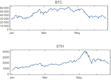
Significant cryptocurrencies
In this section we analyze the summaries of cryptocurrencies data in order to derive a list of the most significant ones.
We choose the phrase “significant cryptocurrency” to mean “a cryptocurrency with high market capitalization, price, or trading volume.”
Together with the summaries we look into the Pareto principle adherence of the corresponding values.
Remark: The Pareto principle adherence should be interpreted carefully here – the cryptocurrencies are not mutually exclusive when in comes to money invested and trading volumes. Nevertheless, we can interpret the corresponding value ratios as indicators of “mind share” or “significance.”
By summaries
Here is a summary of the cryptocurrencies we consider (from Yahoo Finance) ordered by “Market Cap” (largest first):
dsCCSummary = ResourceFunction["CryptocurrencyData"][All, "Summary"]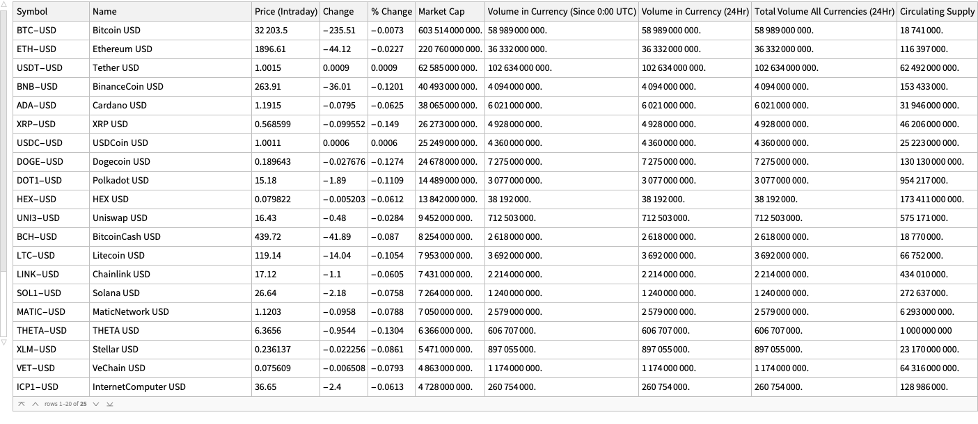
Here is the summary of summary dataset above:
ResourceFunction["RecordsSummary"][dsCCSummary]
Here is a Pareto principle adherence plot for the cryptocurrency market caps:
aMCaps = Normal[dsCCSummary[Association, StringSplit[#Symbol, "-"][[1]] -> #["Market Cap"] &]]; ResourceFunction["ParetoPrinciplePlot"][aMCaps, PlotRange -> All, PlotLabel -> "Pareto principle for cryptocurrency market caps"]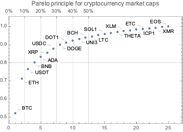
Here is the Pareto statistic for the top 12 cryptocurrencies:
Take[AssociationThread[Keys@aMCaps, Accumulate[Values@aMCaps]]/Total[aMCaps], 12]

(*<|"BTC" -> 0.521221, "ETH" -> 0.71188, "USDT" -> 0.765931, "BNB" -> 0.800902, "ADA" -> 0.833777, "XRP" -> 0.856467, "USDC" -> 0.878274, "DOGE" -> 0.899587, "DOT1" -> 0.9121, "HEX" -> 0.924055, "UNI3" -> 0.932218, "BCH" -> 0.939346|>*)
By price
Get the mean daily closing prices data for the last two weeks and show the corresponding data summary:
startDate = DatePlus[Now, -Quantity[2, "Weeks"]]; aMeans = ReverseSort[Association[# -> Mean[ResourceFunction["CryptocurrencyData"][#, "Close", startDate]["Values"]] & /@ ResourceFunction["CryptocurrencyData"]["Cryptocurrencies"]]];
ResourceFunction["RecordsSummary"][aMeans, Thread -> True]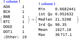
Pareto principle adherence plot:
ResourceFunction["ParetoPrinciplePlot"][aMeans, PlotRange -> All, PlotLabel -> "Pareto principle for cryptocurrency closing prices"]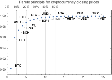
Here are the Pareto statistic values for the top 12 cryptocurrencies:
aCCTop = Take[AssociationThread[Keys@aMeans, Accumulate[Values@aMeans]]/Total[aMeans], 12]

(*<|"BTC" -> 0.902595, "ETH" -> 0.959915, "BCH" -> 0.974031, "BNB" -> 0.982414, "XMR" -> 0.988689, "LTC" -> 0.992604, "FIL" -> 0.99426, "ICP1" -> 0.995683, "ETC" -> 0.997004, "SOL1" -> 0.997906, "LINK" -> 0.998449, "UNI3" -> 0.998987|>*)
Plot the daily closing prices of top cryptocurrencies since January 2018:
DateListPlot[Log10 /@ Association[# -> ResourceFunction["CryptocurrencyData"][#, "Close", "Jan 1, 2018"] & /@ Keys[aCCTop]], PlotLabel -> "lg of crytocurrencies daily closing prices, USD", PlotTheme -> "Detailed", PlotRange -> All]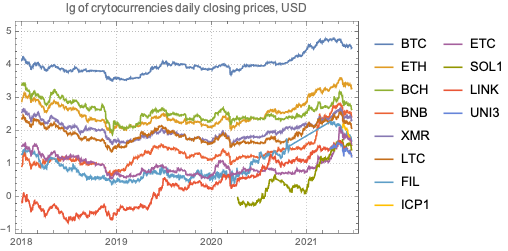
By trading volume
Get the mean daily trading volumes data for the last two weeks and show the corresponding data summary:
startDate = DatePlus[Now, -Quantity[2, "Weeks"]]; aMeans = ReverseSort[Association[# -> Mean[ResourceFunction["CryptocurrencyData"][#, "Volume", startDate]["Values"]] & /@ ResourceFunction["CryptocurrencyData"]["Cryptocurrencies"]]];
ResourceFunction["RecordsSummary"][aMeans, Thread -> True]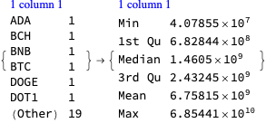
Pareto principle adherence plot:
ResourceFunction["ParetoPrinciplePlot"][aMeans, PlotRange -> {0, 1.1},PlotRange -> All, PlotLabel -> "Pareto principle for cryptocurrency trading volumes"]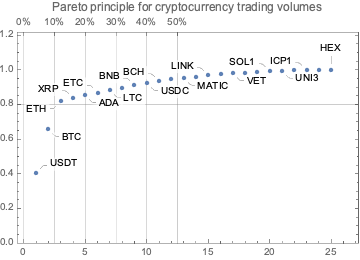
Here are the Pareto statistic values for the top 12 cryptocurrencies:
aCCTop = N@Take[AssociationThread[Keys@aMeans, Accumulate[Values@aMeans]]/Total[aMeans], 12]

(*<|"USDT" -> 0.405697, "BTC" -> 0.657918, "ETH" -> 0.817959, "XRP" -> 0.836729, "ADA" -> 0.853317, "ETC" -> 0.868084, "LTC" -> 0.882358, "DOGE" -> 0.896621, "BNB" -> 0.910013, "USDC" -> 0.923379, "BCH" -> 0.933938, "DOT1" -> 0.944249|>*)
Plot the daily closing prices of top cryptocurrencies since January 2018:
DateListPlot[Log10 /@ Association[# -> ResourceFunction["CryptocurrencyData"][#, "Volume", "Jan 1, 2018"] & /@ Keys[aCCTop]], PlotLabel -> "lg of cryptocurrencies trading volumes", PlotTheme -> "Detailed", PlotRange -> {5, Automatic}]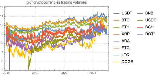
Related events
In this section we make a dataset that has the dates of certain cryptocurrency related events and links to their news announcements.
The events were taken by observing cryptocurrency board stories in the news aggregation site slashdot.org.
lsEventData = {
    {"Jun 18, 2021", "China to shut down over 90% of its Bitcoin mining capacity after local bans", "https://www.globaltimes.cn/page/202106/1226598.shtml"},
    {"Jun 10, 2021", "Global banking regulators call for toughest rules for cryptocurrencies", "https://www.theguardian.com/technology/2021/jun/10/global-banking-regulators-cryptocurrencies-bitcoin"},
    {"June 10, 2021", "IMF sees legal, economic issues with El Salvador's bitcoin move","https://www.reuters.com/business/finance/imf-sees-legal-economic-issues-with-el-salvador-bitcoin-move-2021-06-10/"},
    {"June 8, 2021", "El Salvador Becomes First Country To Adopt Bitcoin as Legal Tender After Passing Law", "https://www.cnbc.com/2021/06/09/el-salvador-proposes-law-to-make-bitcoin-legal-tender.html"},
    {"June 8, 2021", "US recovers millions in cryptocurrency paid to Colonial Pipeline ransomware hackers", "https://edition.cnn.com/2021/06/07/politics/colonial-pipeline-ransomware-recovered/"},
    {"June 4, 2021", "Start of Bitcoin 2021: World\[CloseCurlyQuote]s Largest Cryptocurrency Conference Coming To Wynwood", "https://miami.cbslocal.com/2021/06/04/bitcoin-2021-worlds-largest-cryptocurrency-conference-coming-to-wynwood/"},
    {"June 6, 2021", "End of Bitcoin 2021: World\[CloseCurlyQuote]s Largest Cryptocurrency Conference Coming To Wynwood", "https://miami.cbslocal.com/2021/06/04/bitcoin-2021-worlds-largest-cryptocurrency-conference-coming-to-wynwood/"},
    {"May 28, 2021", "Iran Bans Crypto Mining After Months of Blackouts", "https://gizmodo.com/iran-bans-crypto-mining-after-months-of-blackouts-1846991039"},
    {"May 19, 2021", "Bitcoin, Ethereum prices in free fall as China plans crackdown on mining and trading", "https://www.cnet.com/news/bitcoin-ethereum-prices-in-freefall-as-china-plans-crackdown-on-mining-and-trading/#ftag=CAD590a51e"}
   };
dsEventData = Dataset[lsEventData][All, AssociationThread[{"Date", "Event", "URL"}, #] &];
dsEventData = dsEventData[All, Join[Prepend[#, "DateObject" -> DateObject[#Date]], <|"URL" -> URL[#URL]|>] &];
dsEventData = dsEventData[SortBy[#DateObject &]]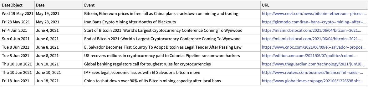
Cryptocurrency time series with events
In this section we discuss possible correlation and causation effects of reported cryptocurrency events.
Remark: The discussion is based on time series and events only, without considering other operational properties of the cryptocurrencies.
Here is a date range:
dateRange = {"May 15 2021", "Jun 21 2021"};Here get time series for the daily opening and closing prices for the selected date range:
aBTCPrices = ResourceFunction["CryptocurrencyData"]["BTC", {"Open", "Close"}, dateRange];
aETHPrices = ResourceFunction["CryptocurrencyData"]["ETH", {"Open", "Close"}, dateRange];
aCCVolume = ResourceFunction["CryptocurrencyData"][{"BTC", "ETH"}, "Volume", dateRange];
Here are the summaries for prices:
ResourceFunction["GridTableForm"][Map[ResourceFunction["RecordsSummary"][#["Values"], "USD"] &, #] & /@ <|"BTC" -> aBTCPrices, "ETH" -> aETHPrices|>]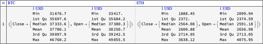
Here are the summaries for trading volumes:
ResourceFunction["RecordsSummary"][#["Values"], "USD"] & /@ aCCVolume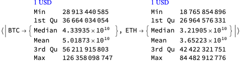
Here we plot the cryptocurrency events with together with the Bitcoin (BTC) price time series:
CryptocurrencyPlot[{aBTCPrices, dsEventData}, PlotLabel -> "BTC daily prices", ImageSize -> 1200]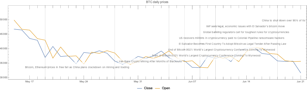
Here we plot the cryptocurrency events with together with the Ether (ETH) price time series:
CryptocurrencyPlot[{aETHPrices, dsEventData}, PlotRange -> {0.95, 1.05} MinMax[aETHPrices[[1]]["Values"]], PlotLabel -> "BTC daily prices", ImageSize -> 1200]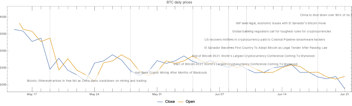
Here we plot the cryptocurrency events with together with the BTC trading volume time series:
CryptocurrencyPlot[{aCCVolume, dsEventData}, PlotLabel -> "BTC and ETH trading volumes", ImageSize -> 1200]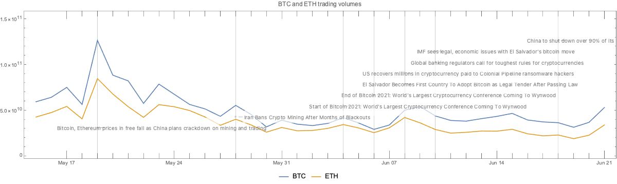
Observations
Going down
We can see that opening prices and volume going down correlate with:
- The news announcement that China plans to crackdown on mining and trading
- The news announcement Iran bans crypto mining
- The Sichuan Provincial Development and Reform Commission and the Sichuan Energy Bureau issue of a joint notice, ordering local electricity companies to “screen, clean up and terminate” mining operations
- The start of the “Bitcoin 2021” conference
Related conjectures:
- We can easily conjecture that 1 and 2 made cryptocurrencies (Bitcoin) less attractive to miners or traders in China and Iran, hence the price and the volume went down.
- The most active Bitcoin traders were attending the “Bitcoin 2021” conference, hence the price and volume went down.
Going up
We can see the prices and volume going up correlate with:
- The news announcement of El Salvador adopting BTC as legal tender currency
- The news announcement that US Justice Department recovered most of the ransom paid to the Colonial Pipeline hackers
- The end of the “Bitcoin 2021” conference
Related conjectures:
- Of course, a country deciding to use BTC as legal tender would make (some) traders willing to invest in BTC.
- The announcement that USA Justice Department, have made (some) traders to more confidently invest in BTC.
- Although, the opposite could also happen – for some people if BTC can be recovered by law enforcement, then BTC is less attractive for financial transactions.
- After the end of “Bitcoin 2021” conference the attending traders resumed their usual activity.
- That conjecture and the “start of Bitcoin 2021” conjecture above support each other.
- The same pattern is observed for both BTC and ETH trading volumes.
Time series correlations
In this section we compute and visualize correlations between the time series of a set of cryptocurrencies.
Getting time series data
Here are the cryptocurrencies we consider:
lsCCFocus = ResourceFunction["CryptocurrencyData"]["Cryptocurrencies"]

(*{"ADA", "BCH", "BNB", "BTC", "DOGE", "DOT1", "EOS", "ETC", "ETH", "FIL", "HEX", "ICP1", "LINK", "LTC", "MATIC", "SOL1", "THETA", "TRX", "UNI3", "USDC", "USDT", "VET", "XLM", "XMR", "XRP"}*)
The start date we use is the one that was 90 days ago:
startDate = DatePlus[Date[], -Quantity[90, "Days"]]

(*{2021, 3, 24, 13, 24, 42.303}*)
aTSOpen = ResourceFunction["CryptocurrencyData"][lsCCFocus, "Open", startDate];
aTSVolume = ResourceFunction["CryptocurrencyData"][lsCCFocus, "Volume", startDate];dateRange = {startDate, Date[]};
aTSOpen2 = Quiet@TimeSeriesResample[#, Append[dateRange, "Day"]] & /@ aTSOpen;
aTSVolume2 = Quiet@TimeSeriesResample[#, Append[dateRange, "Day"]] & /@ aTSVolume;Opening price time series
Show heat-map plot corresponding to the max-normalized time series with clustering:
matVals = Association["SparseMatrix" -> SparseArray[Values@Map[#["Values"]/Max[#["Values"]] &, aTSOpen2]],"RowNames" -> Keys[aTSOpen2], "ColumnNames" -> Range[Length[aTSOpen2[[1]]["Times"]]]];
HeatmapPlot[Map[# /. x_Association :> Keys[x] &, matVals], Dendrogram -> {True, False}, DistanceFunction -> {CosineDistance, None}, ImageSize -> 1200]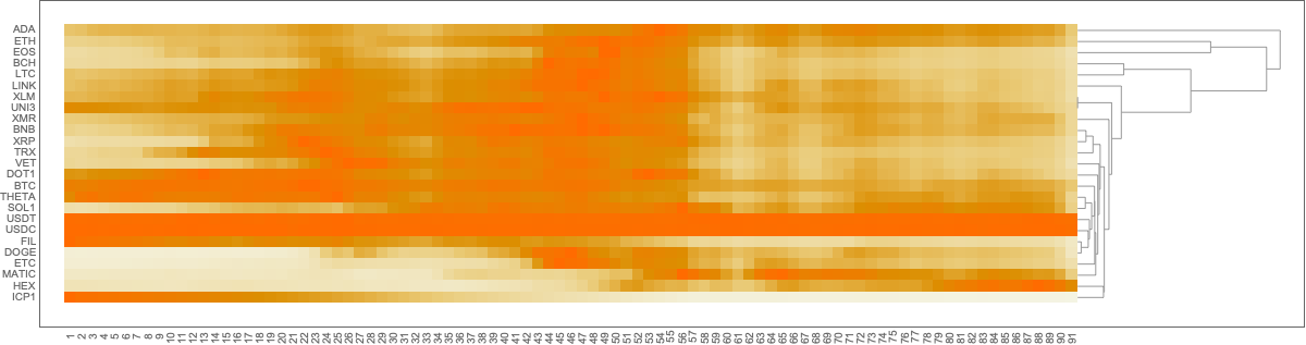
Derive correlation triplets using SpearmanRho :
lsCorTriplets = Flatten[Outer[{#1, #2, SpearmanRho[aTSOpen2[#1]["Values"], aTSOpen2[#2]["Values"]]} &, Keys@aTSOpen2, Keys@aTSOpen2], 1];
dsCorTriplets = Dataset[lsCorTriplets][All, AssociationThread[{"TS1", "TS2", "Correlation"}, #] &];
dsCorTriplets = dsCorTriplets[Select[#TS1 != #TS2 &]];
Show summary of the correlation triplets:
ResourceFunction["RecordsSummary"][dsCorTriplets]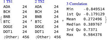
Show correlations that too high or too low:
Dataset[Union[Normal@dsCorTriplets[Select[Abs[#Correlation] > 0.85 &]], "SameTest" -> (Sort[Values@#1] == Sort[Values@#2] &)]][ReverseSortBy[#Correlation &]]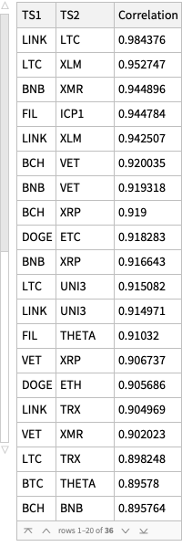
Cross tabulate the correlation triplets and show the corresponding dataset:
dsMatCor = ResourceFunction["CrossTabulate"][dsCorTriplets]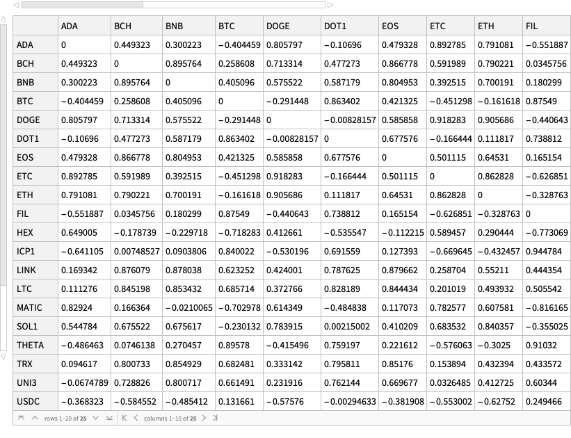
Cross tabulate the correlation triplets and plot the corresponding matrix with heat-map plot:
matCor1 = ResourceFunction["CrossTabulate"][dsCorTriplets, "Sparse" -> True];
gr1 = HeatmapPlot[matCor1, Dendrogram -> {True, True}, DistanceFunction -> {CosineDistance, CosineDistance}, ImageSize -> Medium, PlotLabel -> "Opening price"]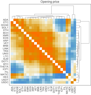
Trading volume time series
Show heat-map plot corresponding to the max-normalized time series with clustering:
matVals = Association["SparseMatrix" -> SparseArray[Values@Map[#["Values"]/Max[#["Values"]] &, aTSVolume2]], "RowNames" -> Keys[aTSOpen2], "ColumnNames" -> Range[Length[aTSVolume2[[1]]["Times"]]]];
HeatmapPlot[Map[# /. x_Association :> Keys[x] &, matVals], Dendrogram -> {True, False}, DistanceFunction -> {CosineDistance, None}, ImageSize -> 1200]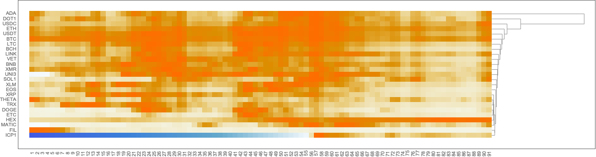
Derive correlation triplets using SpearmanRho :
lsCorTriplets = Flatten[Outer[{#1, #2, SpearmanRho[aTSVolume2[#1]["Values"], aTSVolume2[#2]["Values"]]} &, Keys@aTSVolume2, Keys@aTSVolume2], 1];
dsCorTriplets = Dataset[lsCorTriplets][All, AssociationThread[{"TS1", "TS2", "Correlation"}, #] &];
dsCorTriplets = dsCorTriplets[Select[#TS1 != #TS2 &]];
Show summary of the correlation triplets:
ResourceFunction["RecordsSummary"][dsCorTriplets]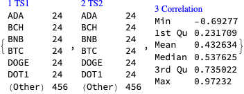
Show correlations that too high or too low:
Dataset[Union[Normal@dsCorTriplets[Select[Abs[#Correlation] > 0.85 &]], "SameTest" -> (Sort[Values@#1] == Sort[Values@#2] &)]][ReverseSortBy[#Correlation &]]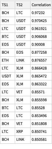
Cross tabulate the correlation triplets and show the corresponding dataset:
dsMatCor = ResourceFunction["CrossTabulate"][dsCorTriplets]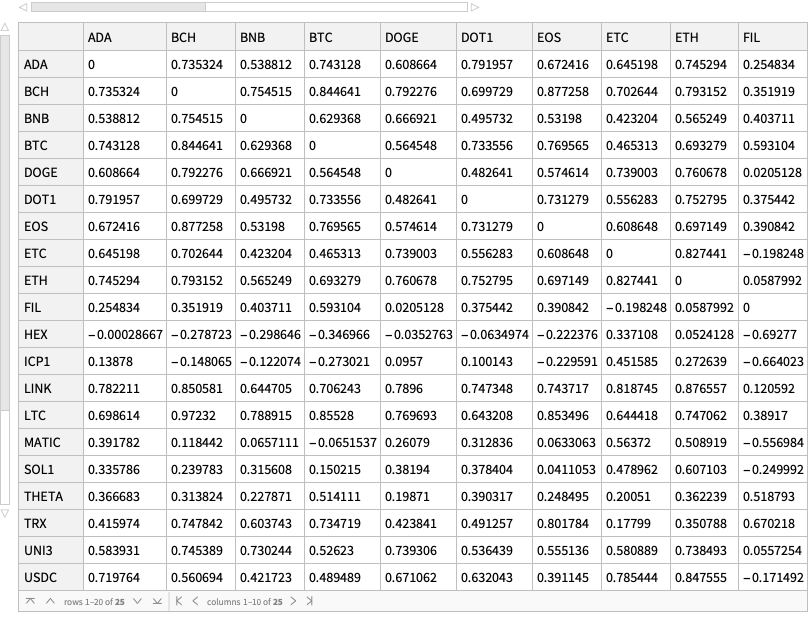
Cross tabulate the correlation triplets and plot the corresponding matrix with heat-map plot:
matCor2 = ResourceFunction["CrossTabulate"][dsCorTriplets, "Sparse" -> True];
gr2 = HeatmapPlot[matCor2, Dendrogram -> {True, True}, DistanceFunction -> {CosineDistance, CosineDistance}, ImageSize -> Medium, PlotLabel -> "Trading volume"]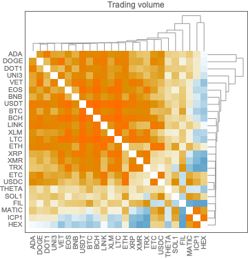
Observations
Here are the correlation matrix plots above placed next to each other:
Row[{gr1, gr2}]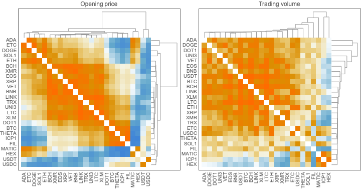
Generally speaking, the two clustering patterns are different. This is one of the reasons to do the nearest neighbor graph clusterings below.
Nearest neighbors graphs
In this section we create nearest neighbor graphs of the correlation matrices computed above and plot clusterings of the nodes.
Graphs overview
Here we create the nearest neighbor graphs:
aNNGraphsVertexRules = Association@MapThread[#2 -> Association[Thread[Rule[Normal[Transpose[#SparseMatrix]], #ColumnNames]]] &, {{matCor1, matCor2}, {"Open", "Volume"}}];aNNGraphs = Association@MapThread[(gr = NearestNeighborGraph[Normal[Transpose[#SparseMatrix]], 4, GraphLayout -> "SpringEmbedding", VertexLabels -> Normal[aNNGraphsVertexRules[#2]]]; #2 -> Graph[EdgeList[gr], VertexLabels -> Normal[aNNGraphsVertexRules[#2]], ImageSize -> Large]) &, {{matCor1, matCor2}, {"Open", "Volume"}}];Here we plot the graphs with clusters:
ResourceFunction["GridTableForm"][List @@@ Normal[CommunityGraphPlot[#, ImageSize -> 800] & /@ aNNGraphs], TableHeadings -> {"Property", "Communities of nearest neighbors graph"}, Background -> White, Dividers -> All]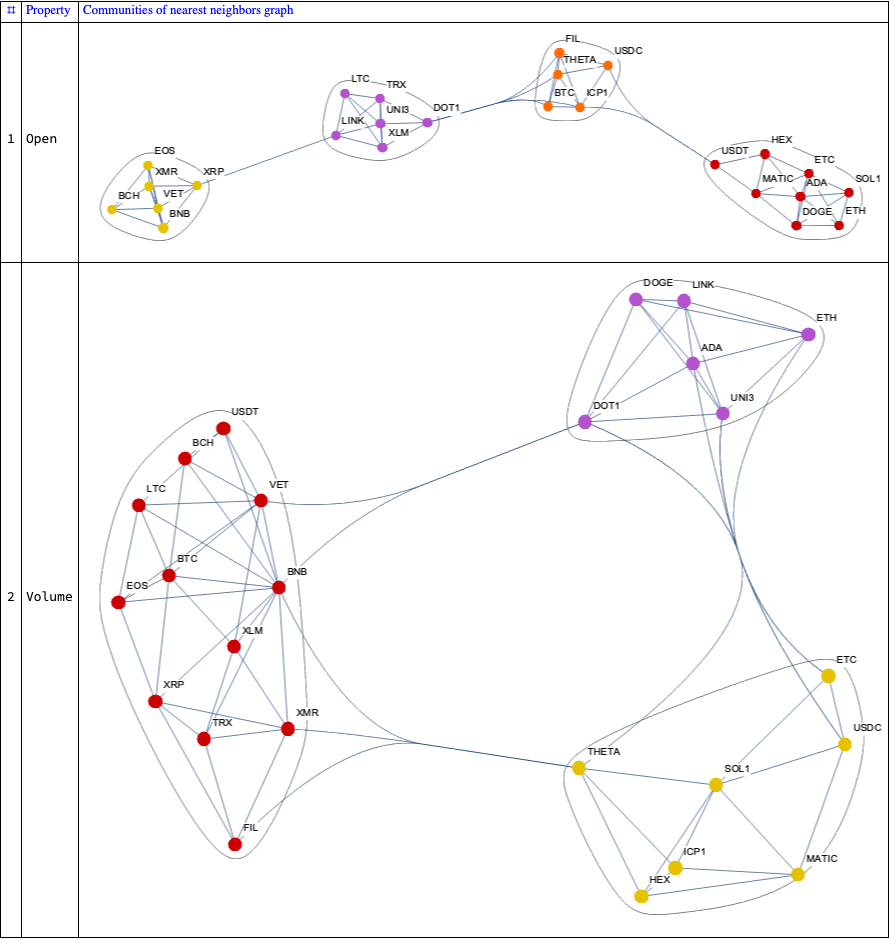
Here are the corresponding time series plots for each cluster:
aClusterPlots =
   Association@Map[
     Function[{prop},
      prop -> Map[
        DateListPlot[Log10 /@ ResourceFunction["CryptocurrencyData"][#, prop, dateRange]] &,
        FindGraphCommunities[aNNGraphs[prop]] /. aNNGraphsVertexRules[prop]]
     ],
     Keys[aNNGraphs]
];ResourceFunction["GridTableForm"][List @@@ Normal[aClusterPlots], TableHeadings -> {"Property", "Cluster plots"}, Background -> White, Dividers -> All]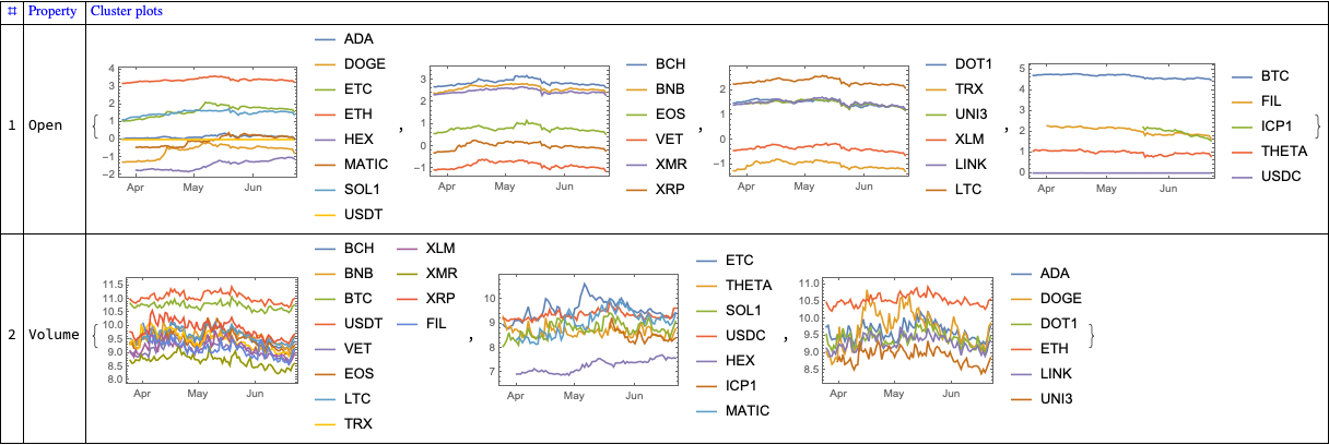
Other types of analysis
I investigated the data with several other methods:
- Clustering with different methods and distance functions
- Clustering after the application of Independent Component Analysis (ICA), [AAw5]
- Time series analysis with Quantile Regression (QR), [AAw6]
None of the outcomes provided some “immediate”, notable insight. The analyses with ICA and QR, though, seem to provide some interesting and fruitful future explorations.
Load packages
Import["https://raw.githubusercontent.com/antononcube/MathematicaForPrediction/master/SSparseMatrix.m"]
Import["https://raw.githubusercontent.com/antononcube/MathematicaForPrediction/master/Misc/HeatmapPlot.m"]
Definitions
Clear[CryptocurrencyPlot];
CryptocurrencyPlot[{aCryptoCurrenciesData_Association, dsEventData_Dataset}, opts : OptionsPattern[]] :=
   Block[{aEventDateObject, aEventURL, aEventRank, grGrid, lsVals},

    aEventDateObject = Normal@dsEventData[Association, {#Event -> AbsoluteTime[#DateObject]} &];
    aEventURL = Normal@dsEventData[Association, {#Event -> Button[Mouseover[Style[#Event, Gray, FontSize -> 10], Style[#Event, Pink, FontSize -> 10]], NotebookLocate[{#URL, None}], Appearance -> None]} &]; aEventRank = Block[{k = 1}, Normal@dsEventData[Association, {#Event -> (k++)/Length[dsEventData]} &]];

    lsVals = Flatten@Map[#["Values"] &, Values@aCryptoCurrenciesData];
    grGrid =
     DateListPlot[
      KeyValueMap[Callout[{#2, Rescale[aEventRank[#1], {0, 1}, MinMax[lsVals]]}, aEventURL[#1], Right] &, Sort@aEventDateObject],
      PlotStyle -> {Gray, Opacity[0.3], PointSize[0.0035]},
      Joined -> False,
      GridLines -> {Sort@Values[aEventDateObject], None}
     ];
    Show[
     DateListPlot[
      aCryptoCurrenciesData,
      opts,
      GridLines -> {Sort@Values[aEventDateObject], None},
      PlotRange -> All,
      AspectRatio -> 1/4,
      ImageSize -> Large
     ],
     grGrid
    ]
   ];
CryptocurrencyPlot[___] := $Failed;
References
Articles
[AA1] Anton Antonov, “Crypto-currencies data acquisition with visualization”, (2021), MathematicaForPrediction at WordPress.
[AA2] Anton Antonov, “NY Times COVID-19 data visualization”, (2020), SystemModeling at GitHub.
[AA3] Anton Antonov, “Apple mobility trends data visualization”, (2020), SystemModeling at GitHub.
Packages
[AAp1] Anton Antonov, Data reshaping Mathematica package, (2018), MathematicaForPrediciton at GitHub.
[AAp2] Anton Antonov, Heatmap plot Mathematica package, (2018), MathematicaForPrediciton at GitHub.
Resource functions
[AAw1] Anton Antonov, CryptocurrencyData, (2021).
[AAw2] Anton Antonov, RecordsSummary, (2019).
[AAw3] Anton Antonov, ParetoPrinciplePlot, (2019).
[AAw4] Anton Antonov, CrossTabulate, (2019).
[AAw5] Anton Antonov, IndependentComponentAnalysis, (2019).
[AAw6] Anton Antonov, QuantileRegression, (2019).

Pingback: Data::Cryptocurrencies | Raku for Prediction