Quantile regression 3D examples

Introduction

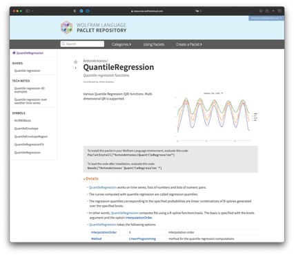
In this notebook we develop in detail Quantile Regression (QR) examples over 3D data via the functions of the paclet “AntonAntonov/QuantileRegression”, [AAp1].

The QR examples demonstrate using:

1. QuantileRegression with “automatic”, NURBS functions (created via BSplineFunction.)

1. QuantileRegressionFit with custom made basis functions

Remark: In order to get a better idea of the how the data looks like, use the 3D graphics interactivity feature rotation.

Remark: This notebook automatically installs the paclet “AntonAntonov/QuantileRegression”, [AAp1] — see the section “Preparation” below.

Remark: A version of this notebook is a technical note in the paclet “AntonAntonov/QuantileRegression” , [AAp1].

---

First neat example

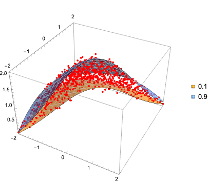
This section has a first neat example with data with triangular domain.

Generate noisy 3D data:

Block[{c = 2, h = 0.1}, 
  data = Flatten[Table[{x, y, Exp[-(x^2 + y^2)/4]*(1 + RandomReal[1.2])}, {x, -c, c, h}, {y, x, c, h}], 1]; 
 ]

Compute Quantile regression for probabilities 0.1 and 0.9 :

probs = {0.1, 0.9};
AbsoluteTiming[
  funcs = AssociationThread[probs -> QuantileRegression[data, 4, probs]]; 
 ]

(*{0.205853, Null}*)

Plot the data points and regression quantiles together:

reg = ConvexHullRegion[Most /@ data];
QRPlot3D[data, funcs, RegionFunction -> Function[{x, y}, RegionMember[reg, {x, y}]]]

---

Noisy arrow wave

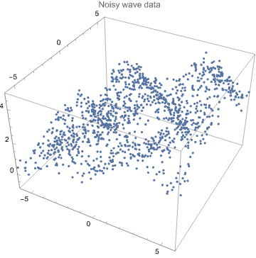
Generate random, “noisy wave” data:

{b, c} = {-6, 6};
data = RandomReal[{b, c}, {1200, 2}];
data = Map[Append[#, Sqrt[#[[1]] - b] + Sin[#[[1]] + Abs[#[[2]]]] + RandomVariate[NormalDistribution[0, 0.3]]] &, data];
Dimensions[data]

(*{1200, 3}*)

3D list plot of the data:

ListPointPlot3D[data, PlotRange -> All, PlotLabel -> "Noisy wave data", BoxRatios -> {1, 1, 2/3}, ImageSize -> Medium]

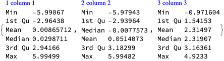
Data summary:

ResourceFunction["RecordsSummary"][data]

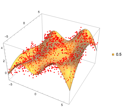
Compute Quantile regression for probability 0.5 using a grid of 7*4 NURBS basis functions:

AbsoluteTiming[
  funcs = QuantileRegression[data, {7, 4}, 0.5]; 
 ]

(*{0.379605, Null}*)

Plot the obtained function and data:

QRPlot3D[data, <|0.5 -> First[funcs]|>]

Quantile regression for probabilities 0.1 and 0.9:

probs = {0.1, 0.9};
AbsoluteTiming[
  funcs = AssociationThread[probs, QuantileRegression[data, {7, 4}, probs]]; 
 ]

(*{0.591367, Null}*)

3D list plot of the data:

QRPlot3D[data, funcs]

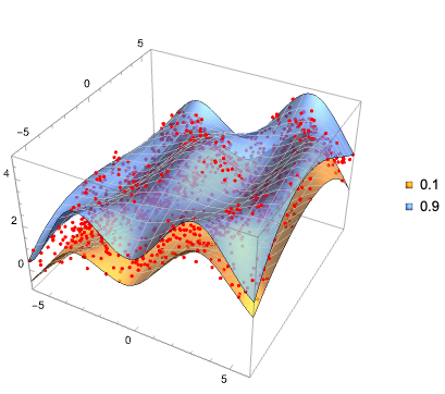
Count the number of points under each surface:

sepPoints = Map[Function[{f}, Length@Select[data, #[[-1]] < First[Apply[f, Most[#]]] &]], funcs]

(*<|0.1 -> 120, 0.9 -> 1087|>*)

Show the corresponding fractions (should correspond to the probabilities):

sepFractions = N[sepPoints/Length[data]]

(*<|0.1 -> 0.1, 0.9 -> 0.905833|>*)

---

Square sombrero

In this section we show the use of QuantileRegressionFit over a pre-generated basis functions.

Remark: The QR computational steps below correspond to the implementation of QuantileRegression .

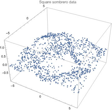
Generate random, “square sombrero” data:

{b, c} = {-6, 6};
data = RandomReal[{b, c}, {1200, 2}];
data = Map[Append[#, Exp[-# . #/(c - b)/2] (Sin[Abs[#[[1]]] + Abs[#[[2]]]] + RandomVariate[NormalDistribution[0, 0.2]])] &, data];
Dimensions[data]

(*{1200, 3}*)

3D list plot of the data:

ListPointPlot3D[data, PlotRange -> All, PlotLabel -> "Square sombrero data", BoxRatios -> {1, 1, 1/1.5}, ImageSize -> Medium]

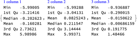
Data summary:

ResourceFunction["RecordsSummary"][data]

NURBS basis of 12*12 functions:

basis = NURBSBasis[data[[All, 1 ;; 2]], 12];
Length[basis]

(*144*)

Quantile regression for probability 0.9:

probs = {0.9};
AbsoluteTiming[
  funcs = AssociationThread[probs, QuantileRegressionFit[data, Through[Values[basis][x, y]], {x, y}, probs]]; 
 ]

(*{6.53867, Null}*)

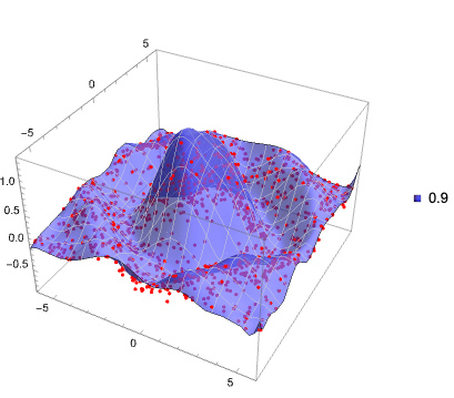
Plot functions and data:

QRPlot3D[data, ToPureFunctions[funcs, {x, y}], ColorFunction -> (Lighter[Blue] &), PlotLegends -> SwatchLegend[{Lighter[Blue]}, Keys[funcs]], Exclusions -> None]

---

Pyramid basis

In this section we demonstrate the use of custom made basis functions.

Define a pyramid basis function:

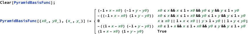
Here is a plot of a basis function:

Plot3D[PyramidBasisFunc[{0, 0}, {x, y}], {x, -1.5, 1.5}, {y, -1.5, 1.5}, PlotRange -> All, ImageSize -> Medium]

Make a basis for the sombrero data:

basis = Flatten@Table[PyramidBasisFunc[{i, j}, {x, y}], {i, b, c}, {j, b, c}];
Length[basis]

(*169*)

Find regression quantiles for probability 0.2:

probs = {0.2};
AbsoluteTiming[
  funcs = 
    AssociationThread[
     probs, QuantileRegressionFit[data, basis, {x, y}, probs, Method -> {LinearProgramming, Method -> "InteriorPoint"}]]; 
 ]

(*{0.866452, Null}*)

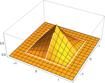
Plot data and regression quantiles together:

QRPlot3D[data, ToPureFunctions[funcs], ColorFunction -> (Lighter[Blue] &), Mesh -> True, PlotLegends -> SwatchLegend[{Lighter[Blue]}, Keys[funcs]], Exclusions -> None]

---

Partial sombrero

In this section we demonstrate the built-in basis filtering in the function NURBSBasis . The basis filtering is used to alleviate (or diminish) fitting problems for data that partially occupies the functional basis domain.

Remark: For a more detailed discussion of how basis filtering is implemented and how it addresses “partial data occupation” problems see the section “Possible issues” of the function page for NURBSBasis .

Generate random, “partial sombrero” data:

{b, c} = {-6, 6};
data = RandomReal[{b, c}, {1600, 2}];
sombreroFunc = Exp[-# . #/(c - b)/4]*Sin[Sqrt[#[[1]]^2 + #[[2]]^2]] &;
data = Map[Append[#, sombreroFunc[##]*(1 + RandomVariate[NormalDistribution[0, 0.6]])] &, data];
Dimensions[data]

(*{1600, 3}*)

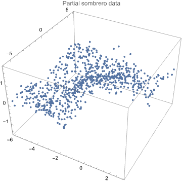
3D list plot of the data:

data2 = Select[data, #[[1]] <= 0.5*#[[2]] &];
ListPointPlot3D[data2, PlotLabel -> "Partial sombrero data", BoxRatios -> {1, 1, 2/3}, ImageSize -> Medium]

Regression quantiles:

probs = {0.1, 0.9};
AbsoluteTiming[
  funcs = AssociationThread[probs, QuantileRegression[data2, 5, probs]]; 
 ]

(*{0.295488, Null}*)

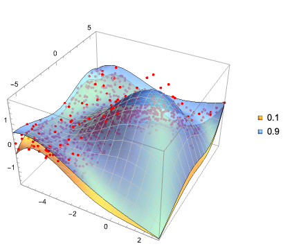
Plot data and regression quantiles together:

QRPlot3D[data2, funcs]

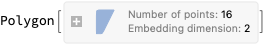
Create a region object for the convex hull of the data points:

reg = ConvexHullRegion[data2[[All, 1 ;; 2]]]

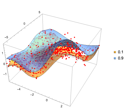
The plot data and regression quantiles over the region above:

QRPlot3D[data2, funcs, RegionFunction -> Function[{x, y}, RegionMember[reg, {x, y}]]]

Count the number of points under each surface:

sepPoints = Map[Function[{f}, Length[Select[data2, #[[-1]] < (f @@ Most[#])[[1]] &]]], funcs]

(*<|0.1 -> 91, 0.9 -> 731|>*)

Show the corresponding fractions (should correspond to the probabilities):

sepFractions = N[sepPoints/Length[data2]]

(*<|0.1 -> 0.112485, 0.9 -> 0.903585|>*)

---

Preparation

Install the paclet:

PacletInstall["AntonAntonov/QuantileRegression"]

Load the Quantile regression paclet:

Needs["AntonAntonov`QuantileRegression`"]

Set random seed:

SeedRandom[9903];

Define plot function:

QRPlot3D[data_List, funcs_Association, opts___] := 
   Show[
    ListPointPlot3D[data, FilterRules[{opts}, {{BoxRatios -> {1, 1, 1/1.5}}}], {BoxRatios -> {1, 1, 1/1.5}}, PlotStyle -> Red, PlotRange -> All], 
    Plot3D[Evaluate@Through[Values[funcs][x, y]], {x, Min[data[[All, 1]]], Max[data[[All, 1]]]}, {y, Min[data[[All, 2]]], Max[data[[All, 2]]]}, 
     opts, 
     PlotRange -> All, PlotStyle -> {Opacity[0.7]}, Mesh -> True, PlotTheme -> "LightMesh", PerformanceGoal -> "Quality", PlotLegends -> Keys[funcs]], ImageSize -> Medium];

Define pure functions converter:

ToPureFunctions[funcs_, vars_List : {x, y}] := 
   Map[With[{f = #}, f &] &, ReplaceAll[funcs, Thread[vars -> Map[Slot, Range[Length[vars]]]]]];

---

References

Articles

[Wk1] Wikipedia entry, Quantile regression.

[Wk2] Wikipedia entry, NURBS.

[AA1] Anton Antonov, “Quantile regression through linear programming”, (2013), MathematicaForPrediction at WordPress.

[AA2] Anton Antonov, “Quantile regression with B-splines”, (2014), MathematicaForPrediction at WordPress.

Books

Roger Koenker, (2005). *Quantile Regression* (Econometric Society Monographs). 2005. Cambridge: Cambridge University Press. doi:10.1017/CBO9780511754098

Functions, packages, paclets

[AAf1] Anton Antonov, QuantileRegression, (2019), Wolfram Function Repository.

[AAp1] Anton Antonov, QuantileRegression paclet, (2023), Wolfram Language Paclet Repository.

[AAp2] Anton Antonov, QuantileRegression Mathematica package, (2013-2023), MathematicaForPrediction at GitHub.

Videos

[AAv1] Anton Antonov, “Quantile Regression—Theory, Implementations, and Applications”, (2014), Wolfram channel at YouTube.